Hello, World!
Week 1 - Introductory Material
Overview
- Syllabus, Objectives & Opener
- Intro to/Foundations of Qualitative Research
- Let’s do some data science!
- Meet the Toolbox
Prepare
Materials
Assignments
- Complete
00-hello_world.qmd, render to PDF and submit to the Class activity submission folder in Google Drive.
Part 1: Syllabus, Objectives & Opener
Part 2: Intro to/Foundations of Qualitative Research
Why wicked problems demand cross-disciplinary methods.
Part 3: Let’s do some data science!
Data Collection
- Yesterday we collected some data from you!
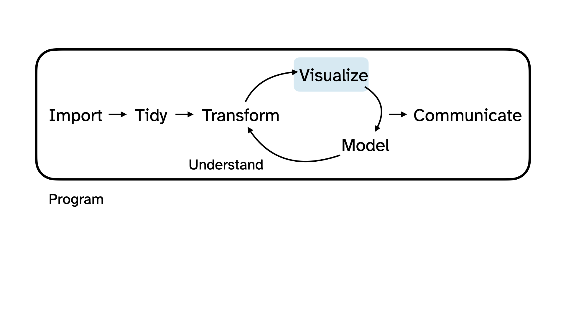
- Today we’re going to explore that data together, following the data science cycle.
- Didn’t take it yet? Scan the QR code and do it now!
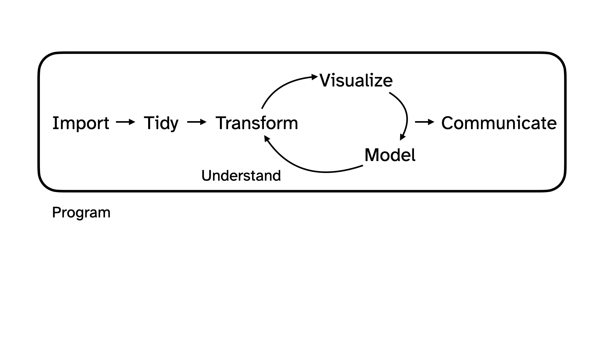
The analysis cycle
You took a survey, built in Google Forms:
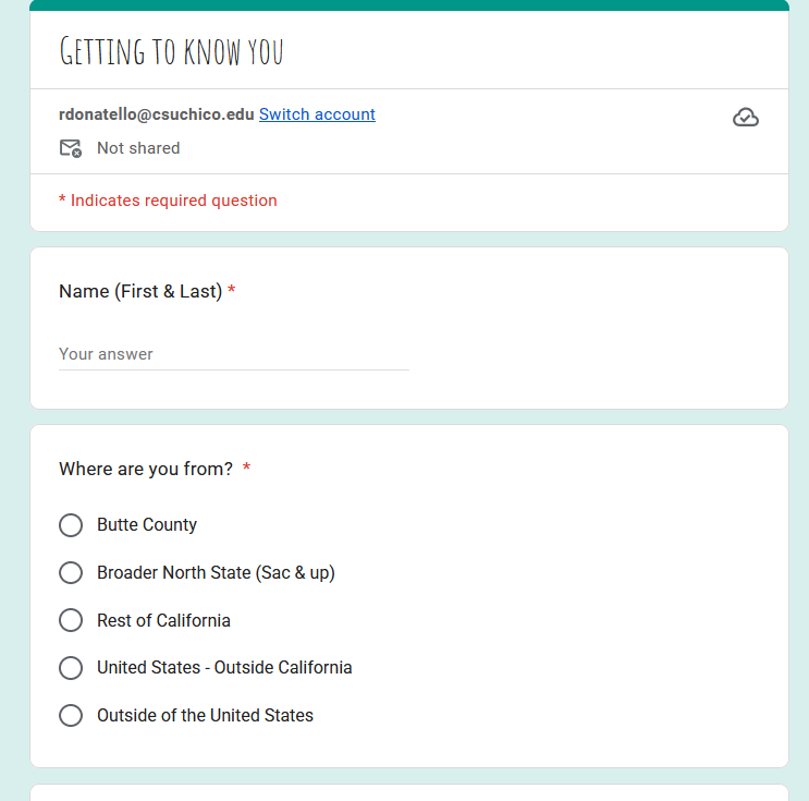
We want to explore that data and get to know you!
Import
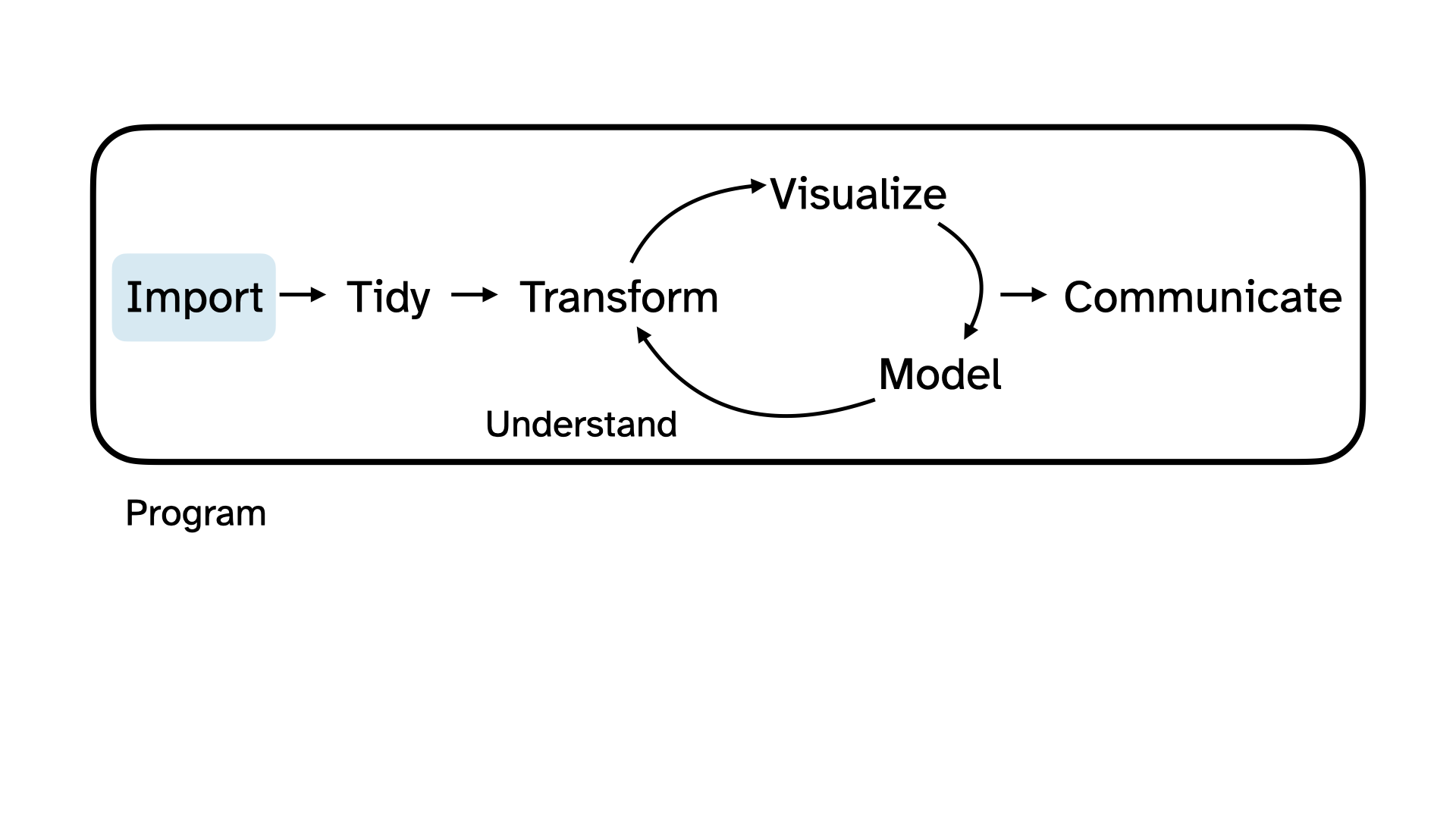
Load some packages
More on what packages are, in a nutshell “get your tools out of the toolbox”.
Import the data
We could download the data and save it as a csv file on our computer, edit out the student names, name it survey-anonymized.csv and save it in a folder called data. Then we would import it into R using the read_csv() function:
Code
survey <- read_csv("data/survey-anonymized.csv")Alternatively, we can authorize R to directly read the Google Sheet that holds the responses from the Google Form you filled out.
Code
survey <- read_sheet("https://docs.google.com/spreadsheets/d/1nUvOJN8z91c3dPN5UrV653qJxlbMCvvj846JDgOscdM")Take a peek at the data
Code
survey# A tibble: 27 × 7
location programming_experience qual_research_experi…¹ qual_data_analysis
<chr> <chr> <chr> <chr>
1 Butte County A little — I’ve writt… A little - for exampl… None
2 Rest of Cal… None Some - I've worked on… A little - for ex…
3 Outside of … None Some - I've worked on… Some - I've worke…
4 Butte County Some — I’ve worked on… Some - I've worked on… A little - for ex…
5 Broader Nor… A little — I’ve writt… A little - for exampl… A little - for ex…
6 Butte County None Some - I've worked on… A little - for ex…
7 Broader Nor… None None None
8 Rest of Cal… None A lot - I've worked o… A lot - I've work…
9 Butte County Some — I’ve worked on… Some - I've worked on… Some - I've worke…
10 Broader Nor… A little — I’ve writt… A little - for exampl… A little - for ex…
# ℹ 17 more rows
# ℹ abbreviated name: ¹qual_research_experience
# ℹ 3 more variables: data_interests <chr>, learn_best <chr>, hopes <chr>Visualize
One way to make sense of data collected is to visualize it.
Multiple Choice Questions
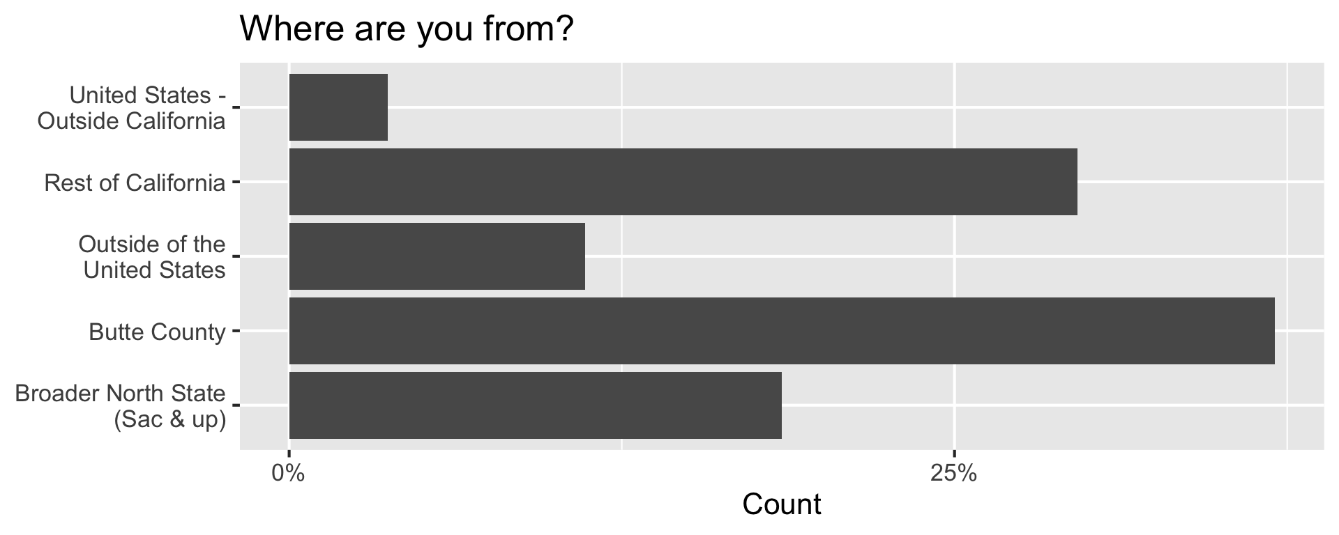
We asked you a couple multiple-choice question where you could only pick one option:
Where are you from?
- Butte County
- Broader North State (Sac & up)
- Rest of California
- United States - Outside California
- Outside of the United States
Code
survey |>
  count(location) |>
  mutate(prop = n / sum(n)) |>
  ggplot(aes(y = location, x = prop))+
  geom_col(show.legend = FALSE) +
  scale_y_discrete(labels = label_wrap(20)) +
  scale_x_continuous(labels = percent_format(accuracy = 1), breaks = c(0, 0.25, 0.5)) +
  labs(
    title = "Where are you from?",
    y = NULL,
    x = "Count"
) 
“How much experience do you have with qualitative research, broadly (e.g. project conceptualization, identifying a sampling strategy, interview instrument design, survey design, data management, etc.)?”
- None
- A little - for example, I have taken a research methods class where we were taught qualitative methods
- Some - I’ve worked on at least one project where I have had to practice some elements of qualitative research
- A lot - I’ve worked on multiple projects where I have gained experience with a variety of qualitative research methods
Code
survey |>
  count(qual_research_experience) |>
  mutate(prop = n / sum(n)) |>
  ggplot(aes(y = fct_reorder(qual_research_experience, prop), x = prop, fill = prop))+
  geom_col(show.legend = FALSE) +
  scale_y_discrete(labels = label_wrap(25)) +
  scale_x_continuous(labels = percent_format(accuracy = 1), breaks = c(0, 0.1, 0.2, 0.3, 0.4)) +
  scale_fill_viridis_c(option = "E") +
  labs(
    title = "Prior qualitative research experience",
    y = NULL,
    x = "Count"
  ) +
  theme_minimal(base_size = 16)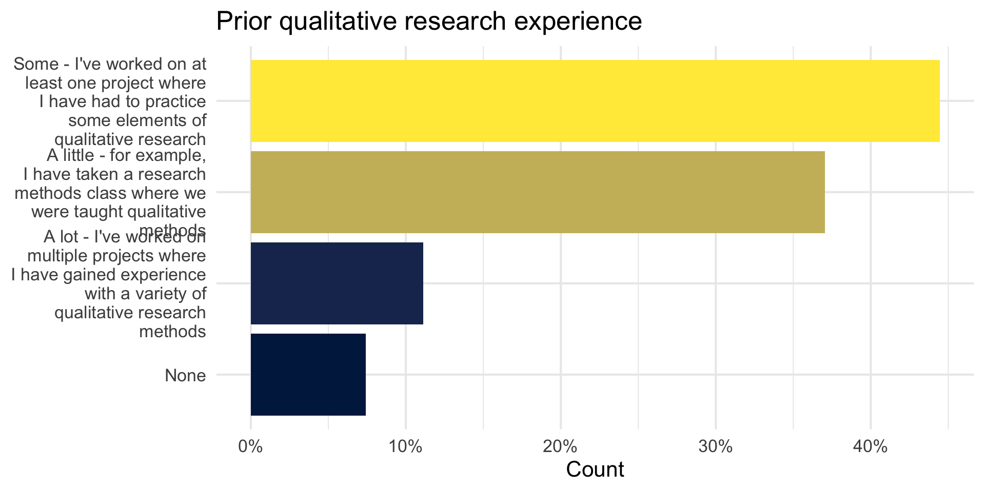
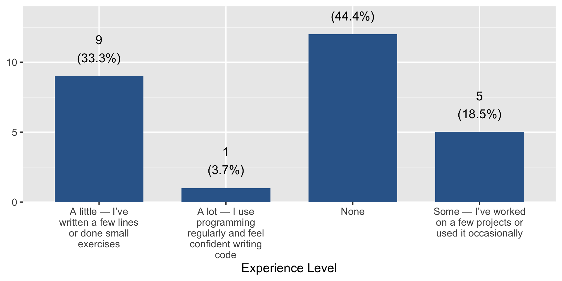
Visualizing data can also reveal trends and set norms.
“How much experience do you have with programming?”
Multiple Answer
We also asked you the following question where you could as many options as you liked:
What types of data interest you?
- Crime
- Economics
- Education
- Entertainment (e.g., books, movies, music)
- Environment/Climate
- Health (e.g., social determinants of health, medical)
- Politics
- Sports
- Other
- No preference
Peek at the data
Code
survey |>
  select(data_interests)
# A tibble: 27 × 1
data_interests
<chr>
1 - Education
2 - Education, - Entertainment (e.g., books, movies, music), - Health (e.g., s…
3 - Environment/Climate, - Health (e.g., social determinants of health, medica…
4 - Education, - Entertainment (e.g., books, movies, music), - Environment/Cli…
5 - Education, - Environment/Climate, - Other
6 - Crime, - Education, - Sports
7 - Economics, - Education, - Environment/Climate, - Health (e.g., social dete…
8 - Other
9 - Health (e.g., social determinants of health, medical), - Politics, - Other
10 - Crime, - Economics, - Education, - Environment/Climate, - Health (e.g., so…
# ℹ 17 more rowsBefore we can visualize this variable, we need to tidy and transform it.
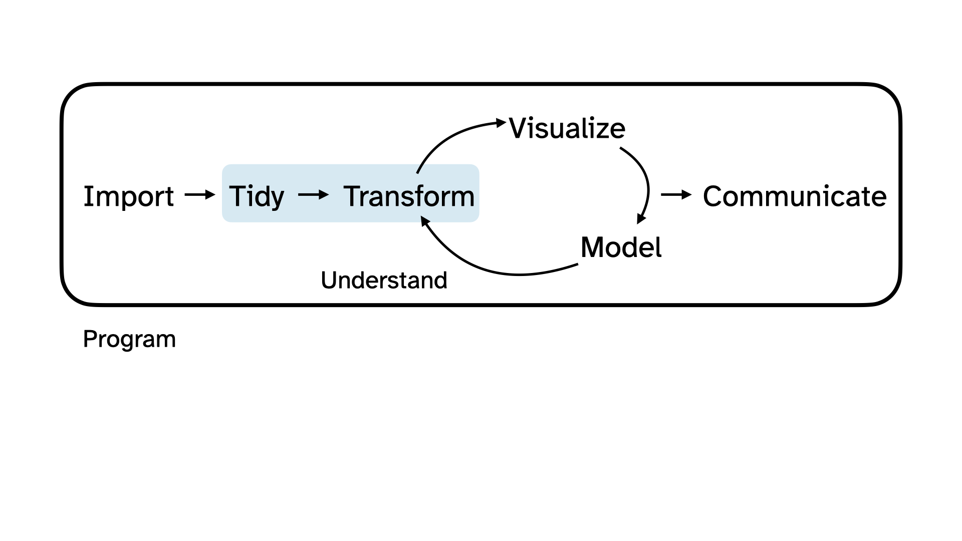
Tidy + Transform
Code
survey |>
  # remove text in parentheses and initial dash
  mutate(data_interests = str_remove_all(data_interests, "\\s*\\(.*?\\)|\\s*-\\s*")) |>
  # separate into multiple rows for each interest, using a semi-colon as delimiter
  separate_longer_delim(data_interests, delim = ",") |>
  mutate(data_interests = trimws(data_interests)) |> # remove leading and trailing spaces
  count(data_interests, sort = TRUE) |>
  mutate(prop = n / sum(n))
# A tibble: 9 × 3
data_interests n prop
<chr> <int> <dbl>
1 Education 20 0.187
2 Health 17 0.159
3 Environment/Climate 16 0.150
4 Politics 15 0.140
5 Crime 11 0.103
6 Entertainment 9 0.0841
7 Economics 8 0.0748
8 Sports 7 0.0654
9 Other 4 0.0374Code
survey |>
  # remove text in parentheses and initial dash
  mutate(data_interests = str_remove_all(data_interests, "\\s*\\(.*?\\)|\\s*-\\s*")) |>
  # separate into multiple rows for each interest, using a semi-colon as delimiter
  separate_longer_delim(data_interests, delim = ",") |>
  mutate(data_interests = trimws(data_interests)) |> # remove leading and trailing spaces
  count(data_interests, sort = TRUE) |>
  mutate(prop = n / sum(n)) |>
  filter(!is.na(data_interests)) |>
  ggplot(aes(y = fct_reorder(data_interests, prop), x = prop, fill = prop)) +
  geom_col(show.legend = FALSE) +
  scale_y_discrete(labels = label_wrap(20)) +
  scale_x_continuous(labels = percent_format(accuracy = 1)) +
  scale_fill_distiller(palette = "RdPu") +
labs(title = "Data interests", y = NULL, x = "Count") 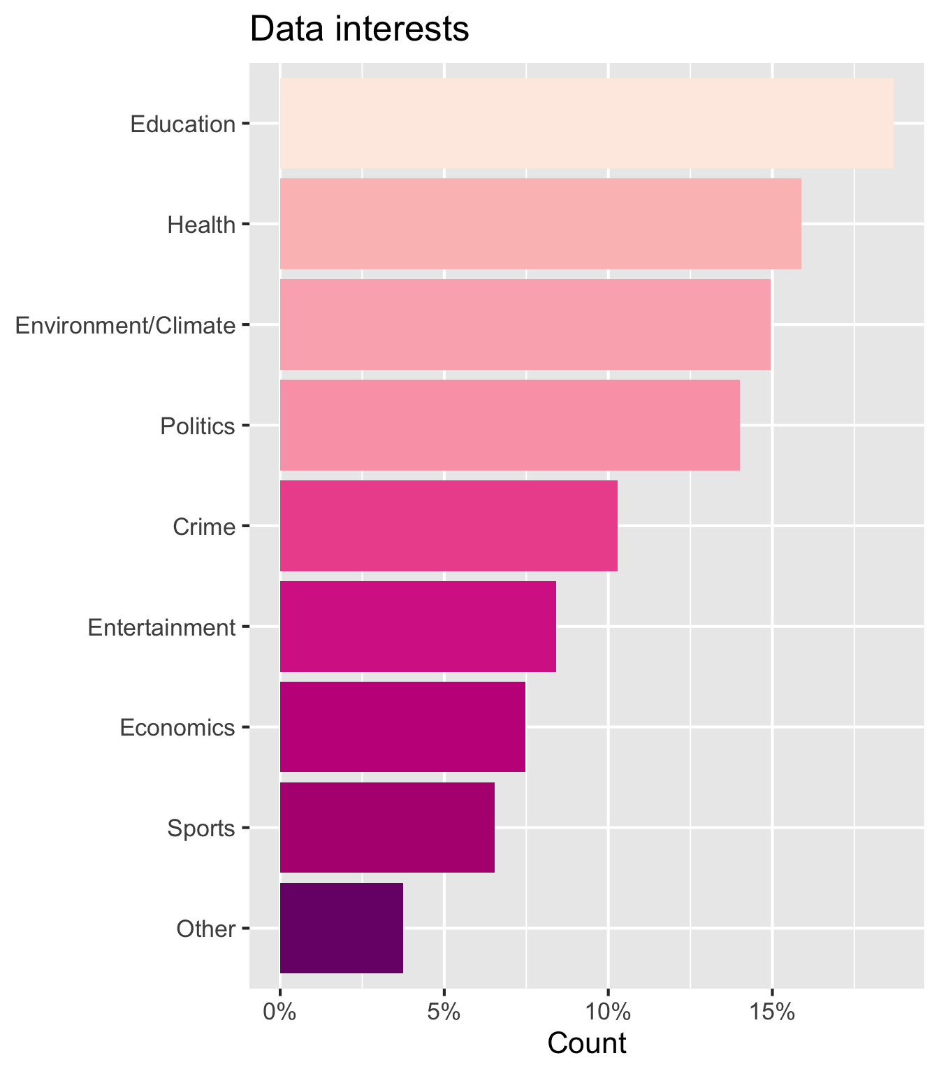
Open Ended
We also asked you a few open-ended questions.
How do you learn best?
Peek at the data
Code
survey |>
  select(learn_best)
# A tibble: 27 × 1
learn_best
<chr>
1 I'm not sure. I like to read about things I'll need to know, but I also try …
2 Solo projects & putting stuff into practice
3 With more smaller assignments rather than fewer larger assignments
4 Hands on activities and learning by observation
5 I learn best from detailed instructions , hands on experience and being abl…
6 Visual learner, with detailed explanations spoken slowly
7 Reading, discussion
8 I like deadlines so I can hold myself accounatble. With coding I might need …
9 I learn best with a mixture of in class discussion, lectures, and readings.
10 I learn best by first listening, then seeing, and finally doing it myself. I…
# ℹ 17 more rowsTidy + Transform + Summarize
We can use text mining techniques, like tokenizing to words to explore this open-ended question:
Code
# A tibble: 9 × 2
  word            n
  <chr>       <int>
1 hands           9
2 learn           7
3 learning        4
4 practice        4
5 visual          4
6 assignments     3
7 class           3
8 learner         3
9 reading         3
We can also tokenize to bigrams (pairs of words):
Code
survey |>
  select(learn_best) |>
  tidytext::unnest_tokens(bigrams, learn_best, token = "ngrams", n = 2) |>
  count(bigrams, sort = TRUE) |>
  filter(n > 2) |>
  print(n = Inf)
# A tibble: 8 × 2
bigrams n
<chr> <int>
1 hands on 9
2 i learn 6
3 learn best 5
4 i am 4
5 best by 3
6 i also 3
7 i can 3
8 visual learner 3It’s a start, but some of these bigrams aren’t helpful. We’d want to remove these to start learning more.
What do you hope to get out of this course?
Not so easy to tidy
And the answers are non-trivial to tidy up, e.g.,
Code
survey$hopes[1:3][1] "I hope to learn more about how to organize and report qualitative data and, if it is appropriate, how to quantify qualitative responses. I'm also interested in learning more about properly gathering and dealing with quantitative data."
[2] "Get more comfortable with statistics and qualitative research."
[3] "Some basic R knowledge and overall improvement in my understanding and confidence with qualitative research methods" Can AI help?
Prompt:
Summarize the following responses to the question “What do you hope to get out of this course?”. Write your response in a short paragraph.
Response:
Students hope to gain stronger skills and confidence in qualitative research methods, including collecting, analyzing, coding, interpreting, and presenting qualitative data. Many also want to improve their understanding of statistics, quantitative analysis, R/RStudio, and data application for research projects, theses, graduate papers, or future PhD work. Overall, they are looking for practical research tools that will help them evaluate studies, conduct their own research, and apply data analysis skills to policy, advocacy, and career goals.
Can it be trusted 100%?
No. They can be misleading, inaccurate, hallucinate or in general sound more confident than they are. Humans should always stay “in the loop”. Hence – the interdisciplinary approach!
Do you have concerns that I gave an AI agent your responses?
Part 4: Meet the Toolbox
Buckle up! You’re going to learn the programming language R, using a program called RStudio, which is installed and fully setup for us inside JupyterHub, which you can access with a web browser.
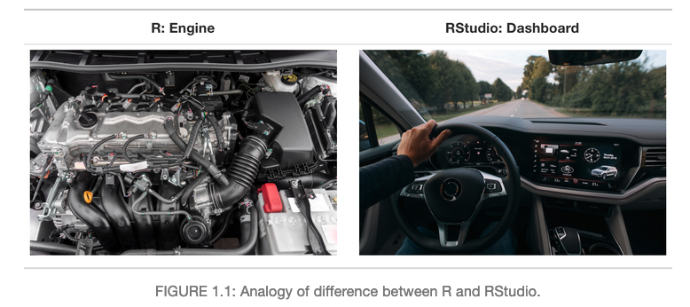
This is where we will create Quarto files that interweave code, output, and narrative text to create a practical reproducible research pipeline that empowers you to be the boss of your own data.
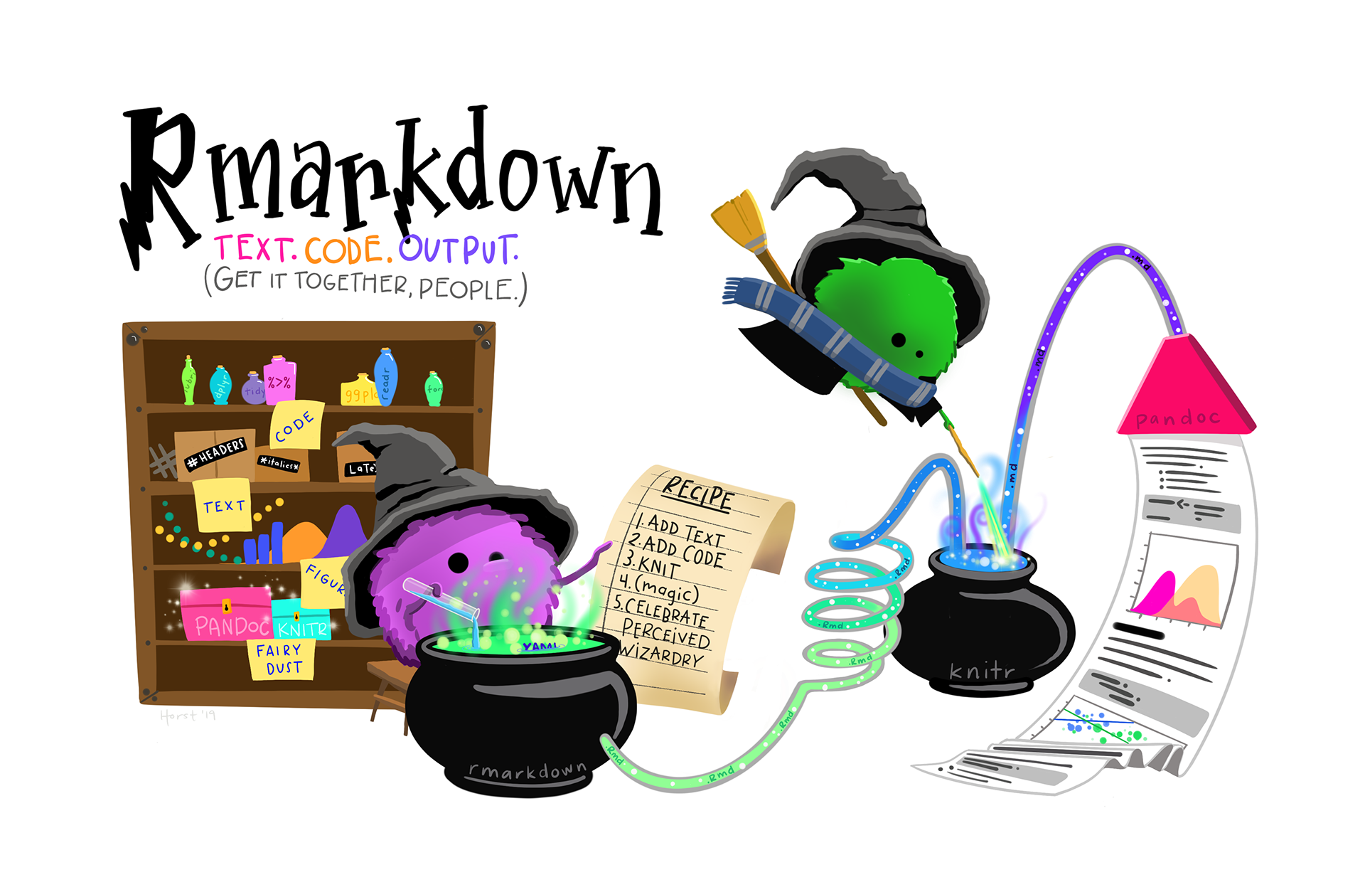
Artwork by Allison Horst
Quarto is the next generation Markdown, but I like this image better
Why this toolkit?
Why R?
- Open source, cross-platform, and free
- Great for reproducibility
- Tons of learning resources
- Works on data of all shapes and sizes
- Produces high-quality graphics
- Large and welcoming community
- Flexible and extensible — doesn’t do something you want? Write a custom function
- Used by professionals across public health, economics and finance, political science and policy research, and social science research — not just academia
Why RStudio?
- Customizable workspace that docks all your windows together
- Notebook formats for easy sharing of code and output
- Syntax highlighting and helpful error warnings
- Cross-platform — works on Windows, macOS, and Linux
- Tab completion for functions — forget the syntax? Popup helpers are there
- One-button publishing of reproducible documents (reports, dashboards, presentations, websites — like this one)
Why JupyterHub?
- No install required — access from any computer with a browser
- Same environment every session — no “it works on my machine” problems
- Log in with your Chico credentials — no extra accounts to manage
- Everyone in class has the same package versions, so troubleshooting is shared, not solo
- Removes setup friction — you’re writing code in minutes, not after an afternoon of installation
Why Quarto?
- One document = narrative + code + output, always in sync — no copy-pasting results into a report
- Fully reproducible — anyone can re-run it and get the same result
- One source file renders to multiple formats (HTML, PDF, Word, slides)
- This course’s entire website is built with it — you’re learning the same tool powering these notes
- The direct successor to R Markdown, with broader language support
Collaborative work - Follow along!
- Log into JupyterHub (will go through SSO)
- Launch Server
- Open RStudio
- In the “Files” pane (lower right corner) Navigate into the “shared/Donatello Wicked” folder
- Click the box next to
00-hello_world.qmd, then “More” and “Copy To”- Click the word “Home” to go back up to your home (root) folder
- Replace the word
worldin the file name with your username (first part of your email). - e.g.
00-hello_rdonatello.qmd
- Back in the “Files” pane, click “Home” to get back to your home directory
- Click on
00-hello_rdonatello.qmdto open this file - Click the “Render”
 button on the top.
 - Make the right side window tall and compare what you see left to right.
Coding is a hands-on activity. You must do your own typing, do your own practice for your brain to connect what you are writing to what it is doing.
Only watching someone code and then trying to do something yourself would be like listening to someone read a book to you and then trying to go write one yourself without being taught how to write.
You try it
- Change the author name in the YAML header to your name
- Try to match the graph colors to the penguin colors
- Answer the remaining questions in the quarto document itself.
Render to PDF and make sure it looks good.
If you don’t finish in class, the rest is homework.
Exporting your file for submission
- In the files tab, click the box next to the PDF for the file you want to export.
- Click “More” –> “Export”
This file will download to your computer. Since it already has your name on it, you can upload it to the Class activity submission folder in Google Drive.
Normalize and accept the struggle
- Hard things make you stronger.
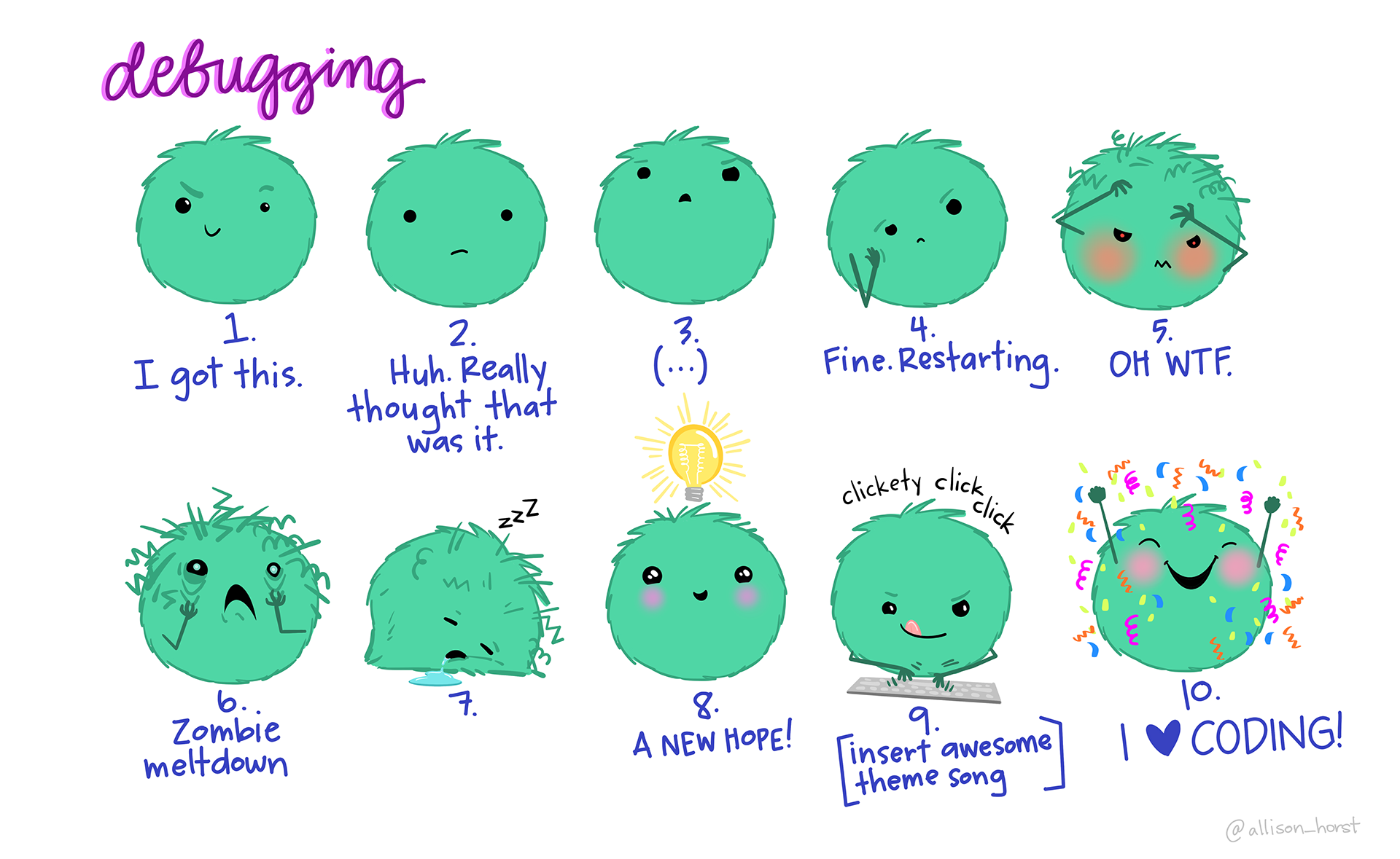
- There is a “roller coaster of emotions” that comes with learning to code is temporary — and normal.
- Learning a programming language is like learning a foreign language: vocabulary, grammar, syntax, and yes — a steep learning curve that takes real commitment. If R feels less comfortable right now than point-and-click tools you’ve used before, that’s expected, not a sign you’re doing something wrong. (R4NP, Ch. 2)
- It’s worth it: R opens up analytical methods that point-and-click software doesn’t have, and the struggle itself builds abstract, conceptual thinking that makes you a stronger researcher — in this class and beyond it.
- Don’t go solo — lean on the learning community.