Topic Modeling

Code along 06

Dr. D

2026-10-12

Packages & Learning objectives

library(tidyverse)   # general data wrangling
library(tidytext)    # text wrangling functions
library(topicmodels) # (NEW!) LDA() and the AssociatedPress data; installs tm along with it

By the end of today, you’ll be able to:

• Describe a document-term matrix (DTM) and what sparse means
• Move between tidy text (one row per token) and a DTM with tidy() and cast_dtm()
• Explain LDA’s two principles and fit a topic model
• Read its two outputs: \(\beta\) (words in a topic) and \(\gamma\) (topics in a document)

Recap: so far we chose the words

• Sentiment: we picked the lexicon, and the lexicon decided which words counted
• N-grams: we picked the word to look into

Today the algorithm proposes the groups of words.

Think of it as a machine’s first pass at open coding: a starting point to check and rename, not a finished codebook.

The Ultimate Goal

This is what we’ve been working towards being able to do all semester. All prior work leads us to the point of being able to use LDA to learn about our text documents in a shorter time frame compared to open coding.

LDA: the birds eye view

LDA (latent Dirichlet allocation) lets an algorithm discover topics in a pile of documents. No labels, no codebook.

• Goes in: a table of word counts per document plus a number of how many topics to look for
• Comes out:
  • topics: lists of words that tend to show up together
  • for each document, how much of each topic it contains
• Left to you: deciding what each topic means

First we look at how to get the text into the necessary shape. Then we fit the model and read what comes out.

TTM 5.1 — Tidying a document-term matrix

What is a document-term matrix?

• one row per document
• one column per term
• each cell is a count

We met the name back in lesson 03: “Four ways to store text.”

A real one: AssociatedPress

data("AssociatedPress")
AssociatedPress

<<DocumentTermMatrix (documents: 2246, terms: 10473)>>
Non-/sparse entries: 302031/23220327
Sparsity           : 99%
Maximal term length: 18
Weighting          : term frequency (tf)

News articles from the Associated Press: each row is an article, each column a word. The header already says Sparsity: 99%. What does that mean?

Sparsity: most cells are 0

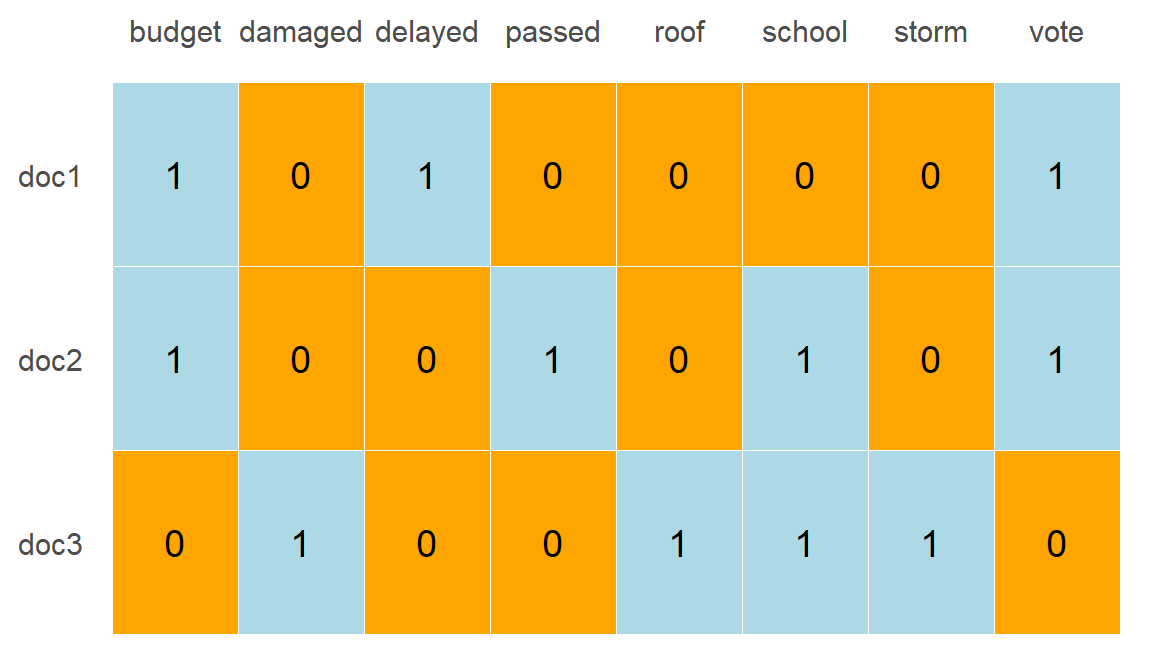
Sparsity = the percent of cells in a matrix that are 0.

A document uses only a few of the words in the whole collection, so every row is mostly zeros.

Sparsity at scale: a corner of AssociatedPress

Full data is 2,246 rows (articles) by 10,473 columns (terms).

Why do we care about sparsity?

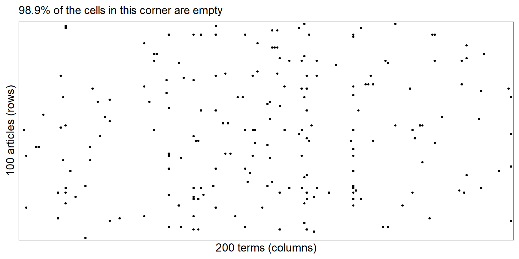
Using the AP data as an example,

n_cells  <- nrow(AssociatedPress) * ncol(AssociatedPress)
n_filled <- length(AssociatedPress$v)   # $v holds only the non-zero counts

tibble(total_cells = n_cells,
       filled      = n_filled,
       empty       = n_cells - n_filled,
       pct_empty   = round(100 * (n_cells - n_filled) / n_cells, 1))

# A tibble: 1 × 4
  total_cells filled    empty pct_empty
        <int>  <int>    <int>     <dbl>
1    23522358 302031 23220327      98.7

• A matrix that stores data from every cell would need 188Mb.
• A sparse matrix stores only the filled cells.
• That is how R keeps a DTM small. A sparse matrix only uses 5.3Mb.

Matrix → tidy: tidy()

Before: the DTM

as.matrix(toy_dtm)

      Terms
Docs   budget delayed vote passed school damaged roof storm
  doc1      1       1    1      0      0       0    0     0
  doc2      1       0    1      1      1       0    0     0
  doc3      0       0    0      0      1       1    1     1

After: tidy()

tidy(toy_dtm)

# A tibble: 11 × 3
   document term    count
   <chr>    <chr>   <dbl>
 1 doc1     budget      1
 2 doc2     budget      1
 3 doc1     delayed     1
 4 doc1     vote        1
 5 doc2     vote        1
 6 doc2     passed      1
 7 doc2     school      1
 8 doc3     school      1
 9 doc3     damaged     1
10 doc3     roof        1
11 doc3     storm       1

Only the filled cells become rows. The zeros are gone.

Matrix → tidy: AssociatedPress

(ap_td <- tidy(AssociatedPress))

# A tibble: 302,031 × 3
   document term       count
      <int> <chr>      <dbl>
 1        1 adding         1
 2        1 adult          2
 3        1 ago            1
 4        1 alcohol        1
 5        1 allegedly      1
 6        1 allen          1
 7        1 apparently     2
 8        1 appeared       1
 9        1 arrested       1
10        1 assault        1
# ℹ 302,021 more rows

• One row per filled cell: 302,031 rows instead of 23.5 million cells.
• Note the column is called term here, where our tidy text used word.

TTM 5.2 — Casting tidy text data into a matrix

Three toy documents → tidy counts

# A tibble: 3 × 2
  document text                                
  <chr>    <chr>                               
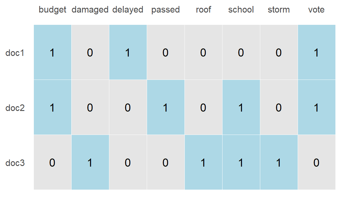
1 doc1     The budget vote was delayed again   
2 doc2     The vote on the school budget passed
3 doc3     The storm damaged the school roof   

toy_counts <- toy_text |>
  unnest_tokens(word, text) |>
  anti_join(stop_words, by = "word") |>
  count(document, word)

# A tibble: 11 × 3
   document word        n
   <chr>    <chr>   <int>
 1 doc1     budget      1
 2 doc1     delayed     1
 3 doc1     vote        1
 4 doc2     budget      1
 5 doc2     passed      1
 6 doc2     school      1
 7 doc2     vote        1
 8 doc3     damaged     1
 9 doc3     roof        1
10 doc3     school      1
11 doc3     storm       1

This is the shape we know from lessons 03 to 05: one row per document-word pair.

Tidy counts → DTM: cast_dtm()

toy_dtm <- toy_counts |>
  cast_dtm(document, word, n)

toy_dtm

<<DocumentTermMatrix (documents: 3, terms: 8)>>
Non-/sparse entries: 11/13
Sparsity           : 54%
Maximal term length: 7
Weighting          : term frequency (tf)

• document → the rows
• word → the columns
• n → the number in each cell

Same counts as the tidy table, now in a grid with the zeros filled back in. This is the shape LDA needs.

🎯 Your turn

Try it yourself

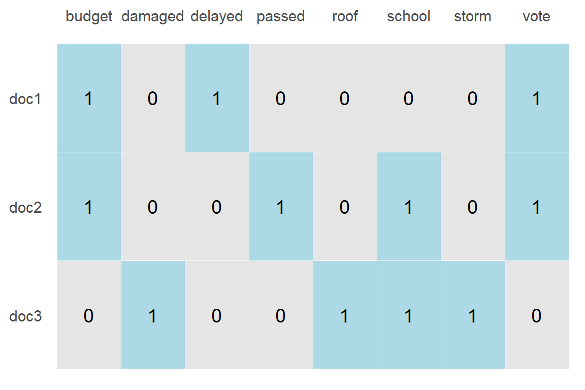
Use the matrix below to answer these questions. Do not use code here. 👀 + 🧠 only

1. Which two documents share the most words? Which words?
2. Does any word appear in all three documents?
3. If we added more documents with new words, would sparsity go up or down?

      Terms
Docs   budget delayed vote passed school damaged roof storm
  doc1      1       1    1      0      0       0    0     0
  doc2      1       0    1      1      1       0    0     0
  doc3      0       0    0      0      1       1    1     1

The workflow

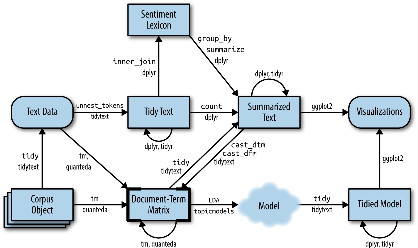
A flowchart of a text analysis that uses topic modeling: the topicmodels package takes a document-term matrix as input and produces a model that tidytext can tidy, so it can be manipulated and visualized with dplyr and ggplot2.

Figure 6.1 from Silge & Robinson, Text Mining with R, used under CC BY-NC-SA 3.0 US.

TTM 6.1 — Latent Dirichlet allocation

Two principles

LDA looks for hidden (“latent”) groups of words. We never observe topics, only the words in the DTM.

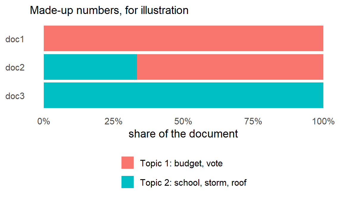
1. Every document is a mixture of topics. One article might be mostly about the budget and a little about schools.

2. Every topic is a mixture of words. And words can be shared: “budget” can matter in both a politics topic and an education topic.

LDA only sees counts, a conceptual bag of words.

Warning: Probability! 😱

	Question it answers	Adds up to 1 across
\(\beta\) (beta)	\(P(\text{word} \mid \text{topic})\): how likely is this word within this topic?	all words, within one topic
\(\gamma\) (gamma)	\(P(\text{topic} \mid \text{document})\): how much of this document comes from this topic?	all topics, within one document

To estimate these probabilities, we use an algorithm containing a random “walk”. A random walk is a series of guesses (estimates) starting at a random point, and iterating until it gets closer (converges) to a value. The Dirichlet probability distribution is what we use to model mixtures like topics and documents.

Zero inflated models are also mixture models.

Fit the model

(ap_lda <- LDA(AssociatedPress, 
               k = 2, 
               control = list(seed = 1234)))

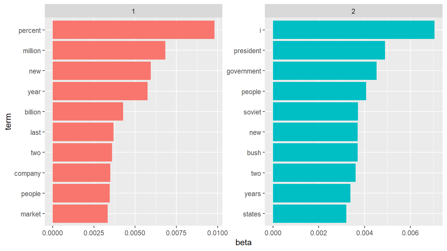
A LDA_VEM topic model with 2 topics.

• k = 2: we choose the number of topics
• seed: LDA starts from a random starting point.

A seed is needed so that everyone’s algorithms start at the same point, resulting in the same answer every time (reproducible).

Different seeds can give different topics. We’ll come back to why, and how to check, at the end.

TTM 6.1.1 Word-topic probabilities (\(\beta\))

ap_topics <- tidy(ap_lda, matrix = "beta")
head(ap_topics)

# A tibble: 6 × 3
  topic term          beta
  <int> <chr>        <dbl>
1     1 aaron     1.69e-12
2     2 aaron     3.90e- 5
3     1 abandon   2.65e- 5
4     2 abandon   3.99e- 5
5     1 abandoned 1.39e- 4
6     2 abandoned 5.88e- 5

• One row per term per topic: 10,473 terms × 2 topics = 20,946 rows
• Read one row: the probability that a word drawn from that topic is that term
• Topic numbers (1, 2) are just labels until we name them

Watch the notation

1.69e-12 is scientific notation for 0.00000000000169

Top terms per topic

1ap_top_terms <- ap_topics |>
  group_by(topic) |>
2  slice_max(beta, n = 10) |>
3  ungroup() |>
  arrange(topic, -beta)

1

within each topic…

2

keep the 10 terms with the largest \(\beta\)

3

ungroup, then sort by topic and \(\beta\)

Top terms per topic

What would you “name” each topic? Remember this data set contains news articles from the AP.

ap_top_terms |>
  mutate(term = reorder_within(term, beta, topic)) |>
  ggplot(aes(beta, term, fill = factor(topic))) +
  geom_col(show.legend = FALSE) +
  facet_wrap(~ topic, scales = "free") +
  scale_y_reordered()

Comparing \(\beta\) across topics

beta_wide <- ap_topics |>
  mutate(topic = paste0("topic", topic)) |>
  # pivot wider to get one row per term, one column per topic
  pivot_wider(names_from = topic, values_from = beta) |> 
  # keep terms common enough in at least one topic to matter
  filter(topic1 > .001 | topic2 > .001) |>
  mutate(log_ratio = log2(topic2 / topic1))

head(beta_wide)

# A tibble: 6 × 4
  term              topic1   topic2 log_ratio
  <chr>              <dbl>    <dbl>     <dbl>
1 administration 0.000431  0.00138      1.68 
2 ago            0.00107   0.000842    -0.339
3 agreement      0.000671  0.00104      0.630
4 aid            0.0000476 0.00105      4.46 
5 air            0.00214   0.000297    -2.85 
6 american       0.00203   0.00168     -0.270

• log2(topic2 / topic1):
  • 0 = word is equally likely in both
  • +1 = word is twice as likely in topic 2
  • −1 = word is half as likely (twice as likely in topic 1)

Interpreting the log2 \(\beta\) ratio

head(beta_wide)

# A tibble: 6 × 4
  term              topic1   topic2 log_ratio
  <chr>              <dbl>    <dbl>     <dbl>
1 administration 0.000431  0.00138      1.68 
2 ago            0.00107   0.000842    -0.339
3 agreement      0.000671  0.00104      0.630
4 aid            0.0000476 0.00105      4.46 
5 air            0.00214   0.000297    -2.85 
6 american       0.00203   0.00168     -0.270

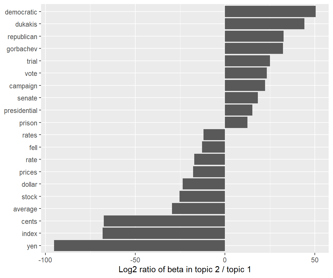
• log2 ratio of +4.46 = \(2^{4.46} = 22\) = 22 times more likely aid is in topic 2 than topic 1
• log2 ratio of -0.27 = \(2^{-0.27} = 0.83\) = 1.2 times more likely that american comes from topic 1 compared to topic 2 (notice we swap which one is more likely due to the sign of the ratio being negative)
• Very large ratios (±30) –> word almost never appears in one of the topics.

Biggest differences

beta_wide |>
  group_by(direction = log_ratio > 0) |>
  slice_max(abs(log_ratio), n = 10) |>
  ungroup() |>
  mutate(term = reorder(term, log_ratio)) |>
  ggplot(aes(log_ratio, term)) +
  geom_col() +
  labs(x = "Log2 ratio of beta in topic 2 / topic 1", y = NULL)

This is a comparative analysis to distinguish topics based on words. Not a reflection on how likely those words are to occur.

dukakis and democrat are pretty much only in topic 2, yen and index in topic 1

\(\beta\) in topic 1 vs. topic 2 - another view

beta_wide |>
  ggplot(aes(topic1, topic2)) +
  geom_abline(slope = 1, intercept = 0, linetype = "dashed", color = "grey50") +
  geom_point(alpha = 0.4) +
  ggrepel::geom_text_repel(
    data = slice_max(beta_wide, pmax(topic1, topic2), n = 20),
    aes(label = term), size = 3) +
  coord_equal() +
  labs(x = expression(beta ~ "in topic 1"), y = expression(beta ~ "in topic 2"))

• Each point is a word (\(\beta\) > .001 in at least one topic)
• On the dashed line: equally likely in both topics
• Near an axis: found almost only in one topic
• Labels: the 20 most common words

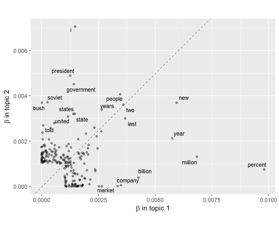
This picture only works for 2 topics. With k > 2 you need one axis per topic, so you’d have to compare topics two at a time.

TTM 6.1.2 Document-topic probabilities (\(\gamma\))

\(\gamma\) is the share of the article’s words that the LDA model estimates came from that topic.

ap_documents <- tidy(ap_lda, matrix = "gamma") # "document" is the response identifier now
head(ap_documents)

# A tibble: 6 × 3
  document topic    gamma
     <int> <int>    <dbl>
1        1     1 0.248   
2        2     1 0.362   
3        3     1 0.527   
4        4     1 0.357   
5        5     1 0.181   
6        6     1 0.000588

• Article 1: \(\gamma\) = 0.25 for topic 1, so about a quarter of its words came from topic 1 (and three quarters from topic 2).
• Article 6: \(\gamma\) = 0.0006 for topic 1, so almost none of its words came from topic 1.

Reading \(\gamma\) across a row

We can use pivot_wider() to create one row per article, one column per topic.

ap_documents |> pivot_wider(names_from = topic, names_prefix = "topic", values_from = gamma) |> head(10)

# A tibble: 10 × 3
   document   topic1 topic2
      <int>    <dbl>  <dbl>
 1        1 0.248    0.752 
 2        2 0.362    0.638 
 3        3 0.527    0.473 
 4        4 0.357    0.643 
 5        5 0.181    0.819 
 6        6 0.000588 0.999 
 7        7 0.773    0.227 
 8        8 0.00445  0.996 
 9        9 0.967    0.0330
10       10 0.147    0.853 

• Each row adds up to 1: that is the article’s mix
• Some articles are clearly on one topic: E.g. articles 6, 8, 9.
• Some articles draw on both topics, so the \(\gamma\) is spread across topics. E.g. articles 1, 2, 3, 4, 5, 7, 10

Picture the mix: 10 AP articles

• Each bar is one article: its \(\gamma\) values stacked to 100%
• One long color: a clean article. Two colors: a blend
• No specific cutoff for clean vs blend.

# name each topic by its top 3 words
topic_labels <- ap_top_terms |>
  group_by(topic) |>
  slice_max(beta, n = 3) |>
  summarize(label = paste(term, collapse = ", ")) |>
  mutate(label = paste0("Topic ", topic, ": ", label))

ap_documents |>
  filter(document <= 10) |>
  left_join(topic_labels, by = "topic") |>
  ggplot(aes(gamma, factor(document), fill = label)) +
  geom_col() +
  scale_y_discrete(limits = rev) +
  scale_x_continuous(labels = scales::percent) +
  guides(fill = guide_legend(nrow = 2)) +
  labs(x = "share of the article", y = "article", fill = NULL) +
  theme_minimal(base_size = 14) +
  theme(legend.position = "bottom", panel.grid = element_blank())

Check the words

ap_td |>
  filter(document == 6) |>
  arrange(desc(count)) |>
  head(10)

# A tibble: 10 × 3
   document term           count
      <int> <chr>          <dbl>
 1        6 noriega           16
 2        6 panama            12
 3        6 jackson            6
 4        6 powell             6
 5        6 administration     5
 6        6 economic           5
 7        6 general            5
 8        6 i                  5
 9        6 panamanian         5
10        6 american           4

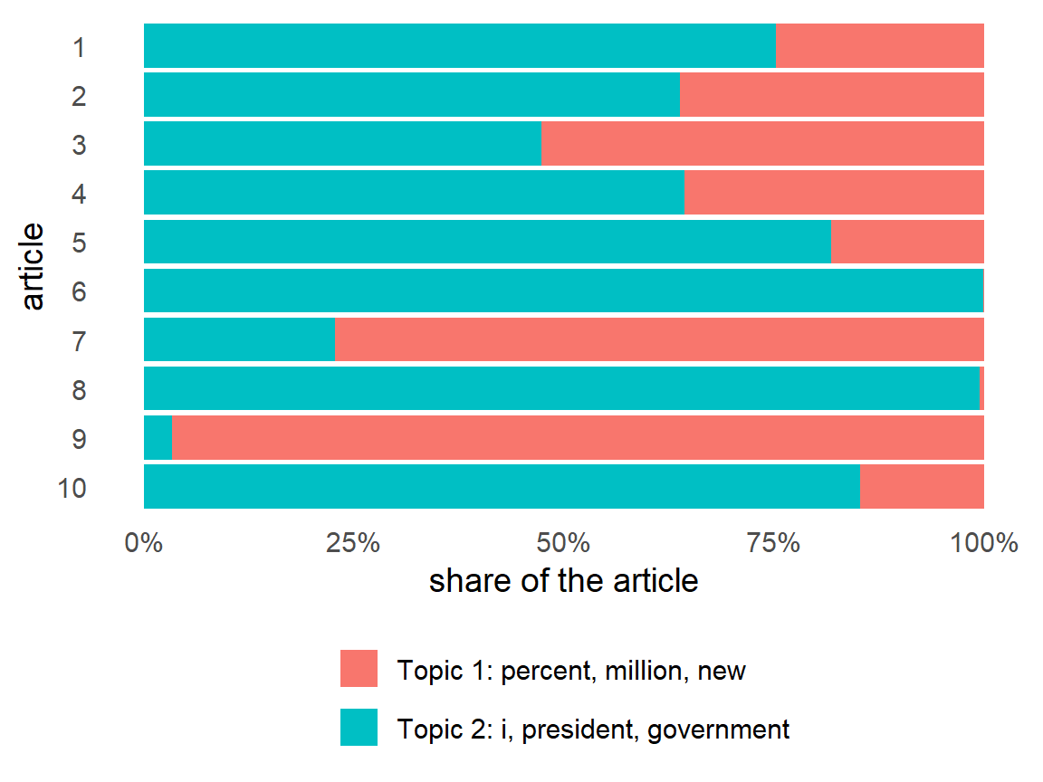
Noriega, Panama, Jackson, Powell: These are all associated with the US invasion of Panama in ’89. Topic 2 may have something to do with invasions?

Same habit: check the words, not just the score.

One label per document: the dominant topic

To help with classification, we can align a document with one specific topic. We can use slice_max(gamma) within each article (document) to keep only the row with the biggest \(\gamma\).

topic_mixture <- ap_documents |>
  group_by(document) |>
  slice_max(gamma)

table(topic_mixture$topic)

   1    2 
 932 1314 

table(topic_mixture$topic) |> prop.table()

        1         2 
0.4149599 0.5850401 

58.5% (n=1314) of all news articles are in Topic 2

Caveat: A label throws away the blend: an article that is 53% topic 1 gets the same label as one that is 97% topic 1.

Visualizing topic networks (Bonus)

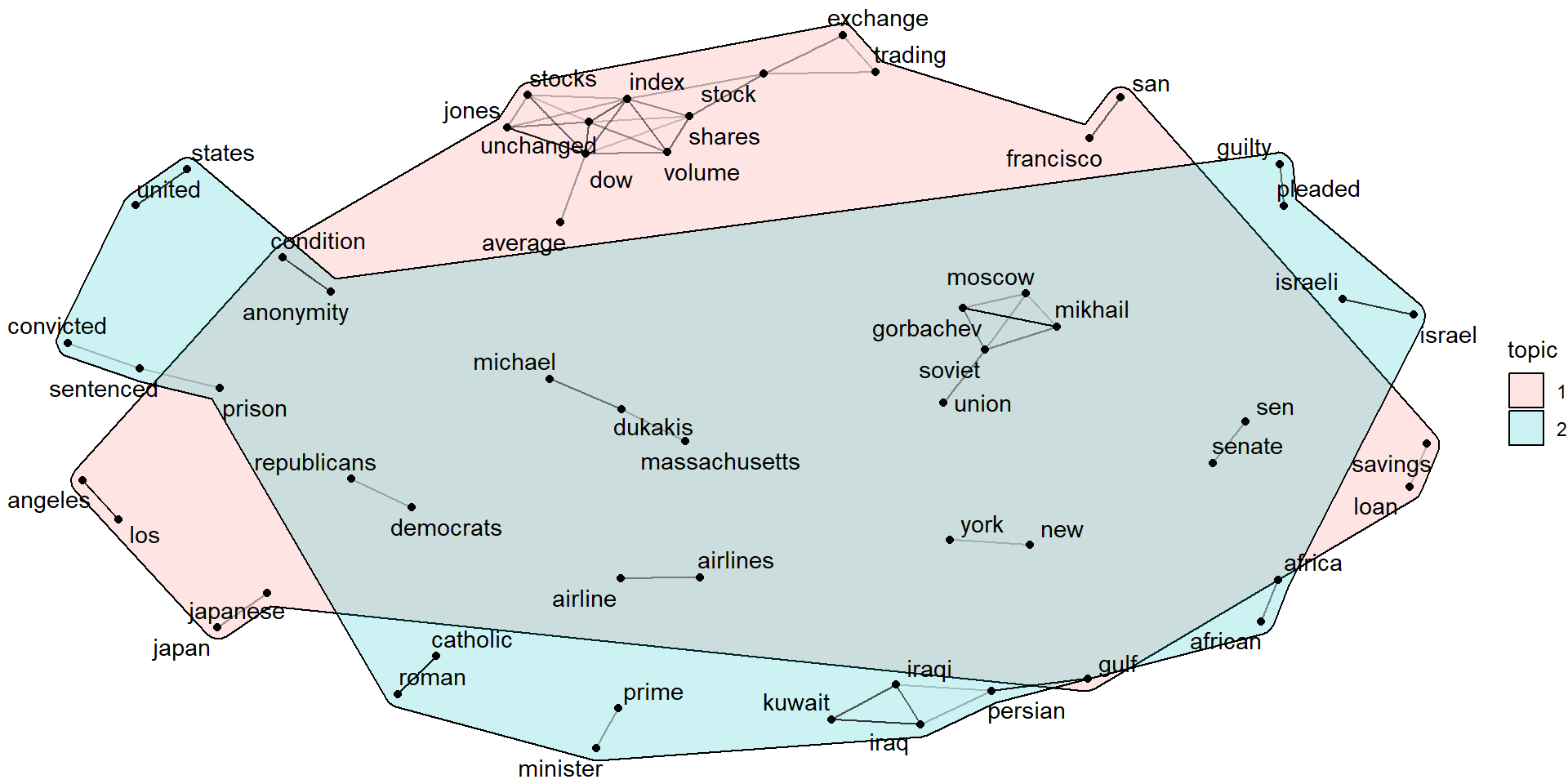
Combining the word correlation network graph, with the topic distribution can shed light on how well our LDA-identified topics cover the topics we can identify from the network graph

library(widyr)   # pairwise_cor(), from lesson 05
library(igraph)  # graph_from_data_frame()
library(ggraph)  # network plot; installs ggforce for the hulls

# topics associated with words
word_topic <- ap_topics |>                  
  group_by(term) |>
  slice_max(beta, n = 1) |> # each word's best topic
  ungroup() |>
  transmute(name = term, topic = factor(topic))

# convert AP dtm to token form
ap_counts <- tidy(AssociatedPress) |>
  count(document, term)


# convert word counts into correlations
cors <- ap_counts |>
  group_by(term) |> filter(sum(n) >= 50) |> ungroup() |>
  pairwise_cor(term, document, sort = TRUE) |>                # same as 05
  filter(correlation > .5)

# create the network graph
g <- graph_from_data_frame(cors, vertices = filter(word_topic, name %in% c(cors$item1, cors$item2)))

# set a seed and add "hulls" 
set.seed(698)
ggraph(g, layout = "fr") +
  ggforce::geom_mark_hull(aes(x, y, group = topic, fill = topic),
                          alpha = .2, concavity = 4, expand = unit(2, "mm")) +
  geom_edge_link(aes(edge_alpha = correlation), show.legend = FALSE) +
  geom_node_point() +
  geom_node_text(aes(label = name), repel = TRUE) +
  theme_void()

Results

What do you notice?

Things I noticed

• Topic 2 has more external countries related to war and possibly war crimes
• Topic 1 is more financial

Trying k = 3

Fit k = 3

(ap_lda3 <- LDA(AssociatedPress,
                k = 3,
                control = list(seed = 1234)))

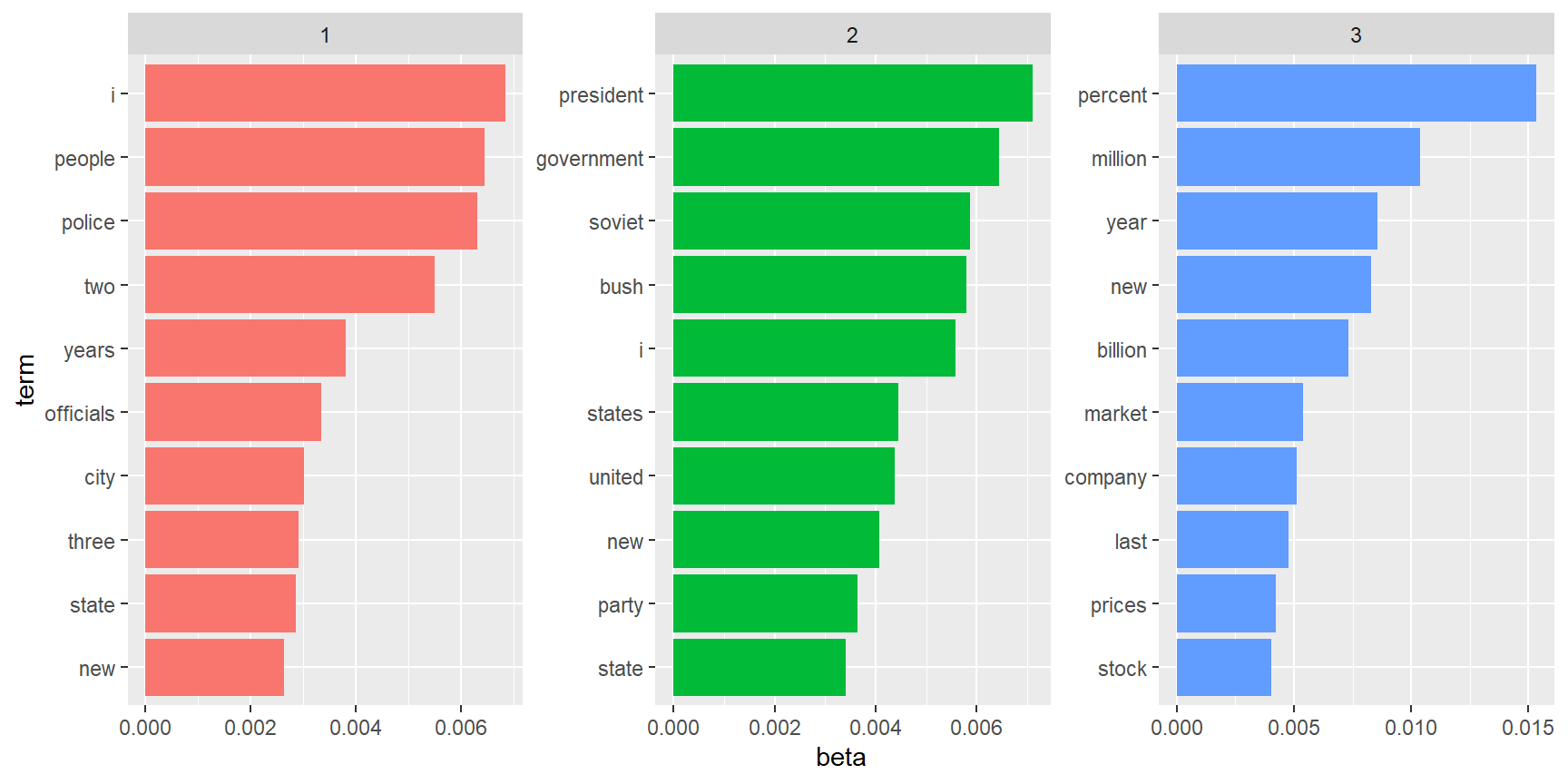
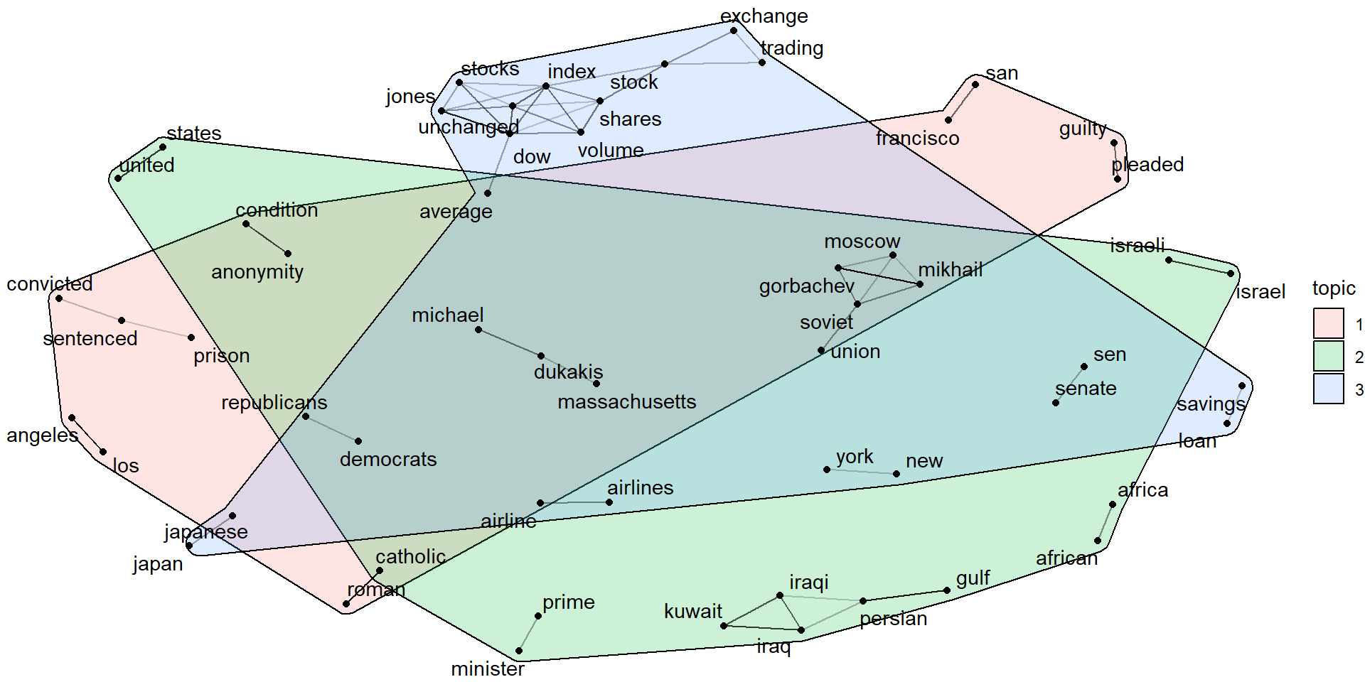
A LDA_VEM topic model with 3 topics.

Same data, same seed, one more topic. The topic number labels (1, 2, 3) are not guaranteed to mean the same thing as before.

Top terms: k = 3

Topic 3 is more clearly economic, but Topic 1 and 2 have some overlap.

ap_topics3 <- tidy(ap_lda3, matrix = "beta")

ap_top_terms3 <- ap_topics3 |>
  group_by(topic) |>
  slice_max(beta, n = 10) |>
  ungroup() |>
  arrange(topic, -beta)

ap_top_terms3 |>
  mutate(term = reorder_within(term, beta, topic)) |>
  ggplot(aes(beta, term, fill = factor(topic))) +
  geom_col(show.legend = FALSE) +
  facet_wrap(~ topic, scales = "free") +
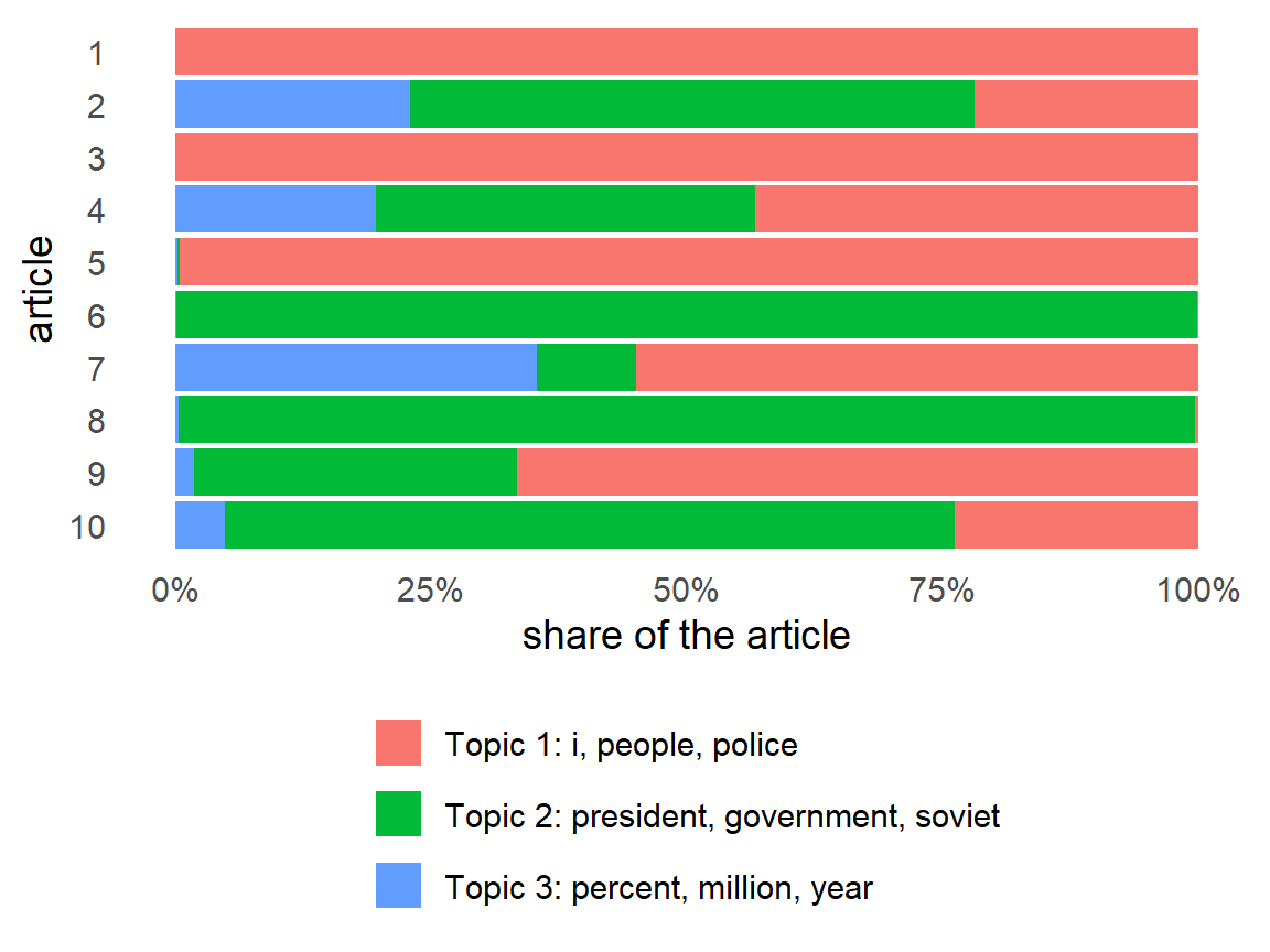
  scale_y_reordered()

Visualize Picture the mix: k = 3

Some articles became more clearly a single topic (e.g. 1, 3, 5, 6, 8)

# name each topic by its top 3 words
topic_labels3 <- ap_top_terms3 |>
  group_by(topic) |>
  slice_max(beta, n = 3) |>
  summarize(label = paste(term, collapse = ", ")) |>
  mutate(label = paste0("Topic ", topic, ": ", label))

tidy(ap_lda3, matrix = "gamma") |>
  filter(document <= 10) |>
  left_join(topic_labels3, by = "topic") |>
  ggplot(aes(gamma, factor(document), fill = label)) +
  geom_col() +
  scale_y_discrete(limits = rev) +
  scale_x_continuous(labels = scales::percent) +
  guides(fill = guide_legend(nrow = 3)) +
  labs(x = "share of the article", y = "article", fill = NULL) +
  theme_minimal(base_size = 14) +
  theme(legend.position = "bottom", panel.grid = element_blank())

Topic hulls: k = 3

Same word network and seed as the k = 2 map, so the words should sit in the same places. Only the topic hulls change.

# each word's best topic, now from the k = 3 model
word_topic3 <- ap_topics3 |>
  group_by(term) |>
  slice_max(beta, n = 1) |>
  ungroup() |>
  transmute(name = term, topic = factor(topic))

# same word correlations (cors) as the k = 2 map
g3 <- graph_from_data_frame(cors, vertices = filter(word_topic3, name %in% c(cors$item1, cors$item2)))

set.seed(321)
ggraph(g3, layout = "fr") +
  ggforce::geom_mark_hull(aes(x, y, group = topic, fill = topic),
                          alpha = .2, concavity = 4, expand = unit(2, "mm")) +
  geom_edge_link(aes(edge_alpha = correlation), show.legend = FALSE) +
  geom_node_point() +
  geom_node_text(aes(label = name), repel = TRUE) +
  theme_void()

Comparing models

Why do different seeds give different topics?

• LDA tries to find the “best” split mathematically.
• The seed only sets LDA’s random starting point
• With only 2 topics, there are several roughly equally good ways to split 2,246 news articles in two: money vs. politics, domestic vs. foreign, and so on
• Different seeds can land on genuinely different splits. That’s a known property of topic models, not a mistake in your code
• Compare top terms, not raw \(\beta\).

Roberts, Stewart & Tingley (2016). “Navigating the Local Modes of Big Data: The Case of Topic Models.” In Computational Social Science: Discovery and Prediction. Cambridge University Press.

Comparing seeds: the topics

Fit the same model with a different seed, then put the top 5 terms side by side.

ap_lda_698 <- LDA(AssociatedPress, k = 2, control = list(seed = 698))

bind_rows(
  tidy(ap_lda, matrix = "beta") |> mutate(seed = 1234),
  tidy(ap_lda_698, matrix = "beta") |> mutate(seed = 698)) |>
  group_by(seed, topic) |>
  slice_max(beta, n = 5) |>
  summarize(top_terms = paste(term, collapse = ", "), .groups = "drop")

# A tibble: 4 × 3
   seed topic top_terms                               
  <dbl> <int> <chr>                                   
1   698     1 percent, million, new, year, bush       
2   698     2 i, people, two, police, government      
3  1234     1 percent, million, new, year, billion    
4  1234     2 i, president, government, people, soviet

Do the topics match? The same two topics with the numbers swapped? Or a different split?

Comparing seeds: the fit

-2*logLik(ap_lda)

'log Lik.' 7163571 (df=20947)

-2*logLik(ap_lda_698)

'log Lik.' 7152762 (df=20947)

• -2*logLik() is a common measure of model fit. The larger the better
• Only comparable for the same \(k\)
• Can let R try several seeds and keep the best (below not run: 5 fits take a few minutes):

ap_lda_best <- LDA(AssociatedPress, k = 2,
                   control = list(nstart = 5, seed = 1:5, best = TRUE))

Comparing k = 2 and k = 3

-2*logLik(ap_lda)

'log Lik.' 7163571 (df=20947)

-2*logLik(ap_lda3)

'log Lik.' 7063461 (df=31420)

• Expect k = 3 to fit better. More topics almost always do, because the model has more room to fit the words
• Compare the topics to choose \(k\):
  • Can you name every topic?
  • Did the extra topic help clarify splits?

Model comparison guidance

1. Set a seed so your results are reproducible
2. Try a few seeds at your k. Keep the one with the highest logLik(), or let nstart + best = TRUE do it
3. Try a few values of k. Keep the one whose topics you can name and defend
4. Check the words: read the top terms and a few example documents, not just the numbers

Recap

• A DTM has one row per document and one column per term; most cells are 0 (sparse)
• tidy() turns a DTM into tidy rows; cast_dtm() turns tidy counts into a DTM
• LDA: documents are mixtures of topics, topics are mixtures of words
• \(\beta\) = words within a topic, \(\gamma\) = topics within a document. You choose k and you name the topics
• Combining LDA topics with a word correlation network graph can uncover patterns and connections you may not have noticed before.