Relationships between words

Code along 05

Dr. D

2026-09-28

Packages & Learning objectives

library(tidyverse)   # general data wrangling
library(tidytext)    # text wrangling functions
library(janeaustenr) # access to her books
library(igraph)      # word network graphs - build it
library(ggraph)      # word network graphs - show it
library(widyr)       # (NEW!) used for analyzing document level co-occurrence

By the end of today, you’ll be able to:

• Tokenize text into bigrams instead of single words
• Use bigram context to catch negation that word-level sentiment misses
• Visualize word relationships as a network graph
• Find co-occurring and correlated words

Recap: one word per row

A couple weeks ago you tokenized text into single words:

austen_books() |>
  unnest_tokens(word, text)

• One token = one word.
• Order is gone — "not happy" becomes two separate rows:
  • "not"
  • "happy"

Remember this caveat?

Last week’s warning about lexicon-based sentiment:

Warning

No negation handling — these are unigram methods. Once “not true” is split into two tokens, “true” just looks true. The qualifier in front of it is invisible to a word-level join.

Today we fix that by capturing word order.

• Instead of tokenizing into single words, we tokenize into overlapping pairs of words
• Two consecutive words = a bigram
• Now "not happy" stays together as one token

4.1 — Tokenizing by n-grams

From words to bigrams

Add token = "ngrams" and n = 2 to unnest_tokens():

austen_bigrams <- austen_books() |>
  unnest_tokens(bigram, text, token = "ngrams", n = 2) |>
  filter(!is.na(bigram))

head(austen_bigrams)

# A tibble: 6 × 2
  book                bigram         
  <fct>               <chr>          
1 Sense & Sensibility sense and      
2 Sense & Sensibility and sensibility
3 Sense & Sensibility by jane        
4 Sense & Sensibility jane austen    
5 Sense & Sensibility chapter 1      
6 Sense & Sensibility the family     

Notice the overlap: “sense and” is one token, “and sensibility” is another.

Most common bigrams

austen_bigrams |>
  count(bigram, sort = TRUE)

# A tibble: 193,209 × 2
   bigram       n
   <chr>    <int>
 1 of the    2853
 2 to be     2670
 3 in the    2221
 4 it was    1691
 5 i am      1485
 6 she had   1405
 7 of her    1363
 8 to the    1315
 9 she was   1309
10 had been  1206
# ℹ 193,199 more rows

Same problem as single words — the top of the list is stop-word pairs: “of the”, “to be”, “in the”.

Splitting and filtering (step by step)

1bigrams_separated <- austen_bigrams |>
  separate(bigram, c("word1", "word2"), sep = " ", remove = FALSE)

2bigrams_filtered <- bigrams_separated |>
  filter(!word1 %in% stop_words$word) |>
  filter(!word2 %in% stop_words$word)

3bigram_counts <- bigrams_filtered |>
  count(word1, word2, sort = TRUE)

1

separate the bigram variable into two variables (word1 and word2) using a space delimiter, but don’t remove the original variable (remove = FALSE).

2

remove rows that have a stopword in either word1 or word2

3

count the remaining bigrams

Splitting and filtering

head(bigram_counts)

# A tibble: 6 × 3
  word1   word2         n
  <chr>   <chr>     <int>
1 sir     thomas      266
2 miss    crawford    196
3 captain wentworth   143
4 miss    woodhouse   143
5 frank   churchill   114
6 lady    russell     110

Names dominate once stop words are gone: “sir thomas”, “miss crawford”, “captain wentworth”.

Streets of Austen

Which streets get mentioned in each book?

bigrams_filtered |>                  # start with the filtered books
  filter(word2 == "street") |>       # keep rows where the second word is 'street'
  count(book, word1, sort = TRUE)    # count the occurrences of word 1

# A tibble: 33 × 3
   book                word1           n
   <fct>               <chr>       <int>
 1 Sense & Sensibility harley         16
 2 Sense & Sensibility berkeley       15
 3 Northanger Abbey    milsom         10
 4 Northanger Abbey    pulteney       10
 5 Mansfield Park      wimpole         9
 6 Pride & Prejudice   gracechurch     8
 7 Persuasion          milsom          5
 8 Sense & Sensibility bond            4
 9 Sense & Sensibility conduit         4
10 Persuasion          rivers          4
# ℹ 23 more rows

🎯 Your turn

Try it yourself

Pick your own word for word2 and see what turns up. Try something like "park", or any word you’re curious about.

bigrams_filtered |>
  filter(word2 == "your word here") |>
  count(book, word1, sort = TRUE)

You could also choose to filter on word1 and count the frequency of word2. Your choice!

Share out: What did you find?

4.2 — Bigrams give context

Words following “not”

bigrams_separated |>
  filter(word1 == "not") |>
  count(word1, word2, sort = TRUE)

# A tibble: 1,178 × 3
   word1 word2     n
   <chr> <chr> <int>
 1 not   be      580
 2 not   to      335
 3 not   have    307
 4 not   know    237
 5 not   a       184
 6 not   think   162
 7 not   been    151
 8 not   the     135
 9 not   at      126
10 not   in      110
# ℹ 1,168 more rows

Discussion: "not" is in the standard stop_words list. Why did we start from bigrams_separated here instead of bigrams_filtered?

Removing stopwords first would have deleted the word "not" itself, before we ever got the chance to search for it.

Joining sentiment to bigrams

AFINN <- get_sentiments("afinn")                    # import lexicon

not_words <- bigrams_separated |>                   
  filter(word1 == "not") |>                         # keep 'not' bigrams
  inner_join(AFINN, by = c(word2 = "word")) |>      # apply sentiment
  count(word1, word2, value, sort = TRUE)           # count

head(not_words)

# A tibble: 6 × 4
  word1 word2 value     n
  <chr> <chr> <dbl> <int>
1 not   like      2    95
2 not   help      2    77
3 not   want      1    41
4 not   wish      1    39
5 not   allow     1    30
6 not   care      2    21

The most common sentiment word after “not” is “like” — normally scored +2.

Plot: what “not” flips

Weight each word by how often it appears and how strong the score:

not_words |>
  mutate(contribution = n * value) |>
  arrange(desc(abs(contribution))) |>
  head(20) |>
  mutate(word2 = reorder(word2, contribution)) |>
  ggplot(aes(n * value, word2, fill = n * value > 0)) +
  geom_col(show.legend = FALSE) +
  labs(x = "Sentiment value × number of occurrences",
       y = "Words preceded by \"not\"")

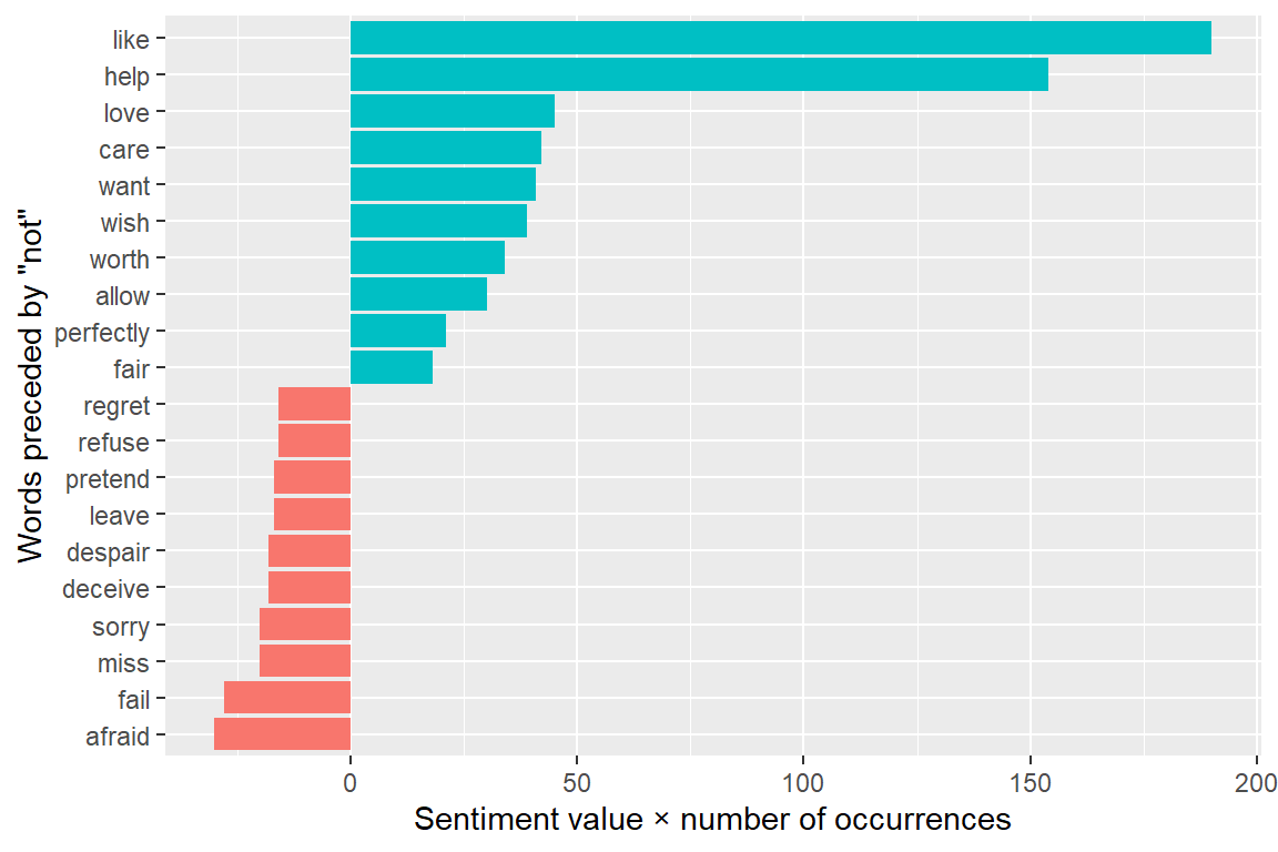
“not like” and “not help” are the biggest mistakes. They make the text look far more positive than it is.

🎯 Your turn

Try it yourself

“Not” isn’t the only negator. Repeat the same join-and-count approach (slide 14) for a vector of negation words instead of a single “not”. Some starter code has been provided.

negation_words <- c("not", "no", "never", "without")

Multiple negation words

negation_words <- c("not", "no", "never", "without")

negated_words <- bigrams_separated |>
  filter(word1 %in% negation_words) |>
  inner_join(AFINN, by = c(word2 = "word")) |>
  count(word1, word2, value, sort = TRUE)

head(negated_words)

# A tibble: 6 × 4
  word1 word2 value     n
  <chr> <chr> <dbl> <int>
1 no    doubt    -1    96
2 not   like      2    95
3 not   help      2    77
4 no    no       -1    58
5 not   want      1    41
6 not   wish      1    39

Visualize to learn more

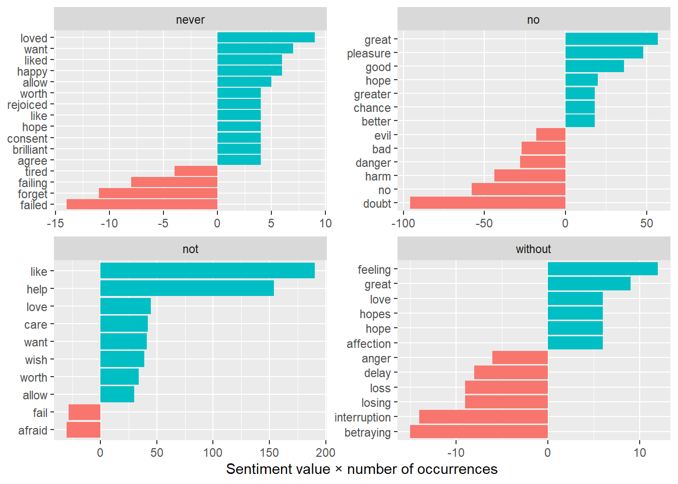
• Still see “not like” and “not help”, but also “no great” and “never loved.”
• We could combine this with the approach in Chapter 2 to reverse the AFINN values of each word that follows a negation (positive –> negative).

4.3 — Visualizing word networks

From pairs to a network (a “toy” example)

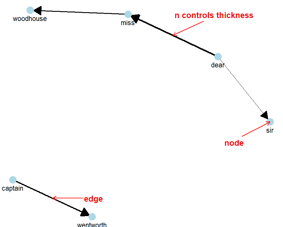
toy_edges

# A tibble: 4 × 3
  from    to            n
  <chr>   <chr>     <dbl>
1 dear    miss          8
2 dear    sir           3
3 miss    woodhouse     5
4 captain wentworth     6

A graph is tidy data with three columns:

• from — the node an edge starts at
• to — the node an edge points to
• n — the frequency of this bigram

Building the graph object

The igraph package turns an edge list into a graph:

bigram_graph <- bigram_counts |>
  filter(n > 20) |>
  graph_from_data_frame()

bigram_graph

IGRAPH dbd1ee1 DN-- 85 70 -- 
+ attr: name (v/c), n (e/n)
+ edges from dbd1ee1 (vertex names):
 [1] sir     ->thomas     miss    ->crawford   captain ->wentworth 
 [4] miss    ->woodhouse  frank   ->churchill  lady    ->russell   
 [7] sir     ->walter     lady    ->bertram    miss    ->fairfax   
[10] colonel ->brandon    sir     ->john       miss    ->bates     
[13] jane    ->fairfax    lady    ->catherine  lady    ->middleton 
[16] miss    ->tilney     miss    ->bingley    thousand->pounds    
[19] miss    ->dashwood   dear    ->miss       miss    ->bennet    
[22] miss    ->morland    captain ->benwick    miss    ->smith     
+ ... omitted several edges

Building the graph

and the ggraph package makes the plot.

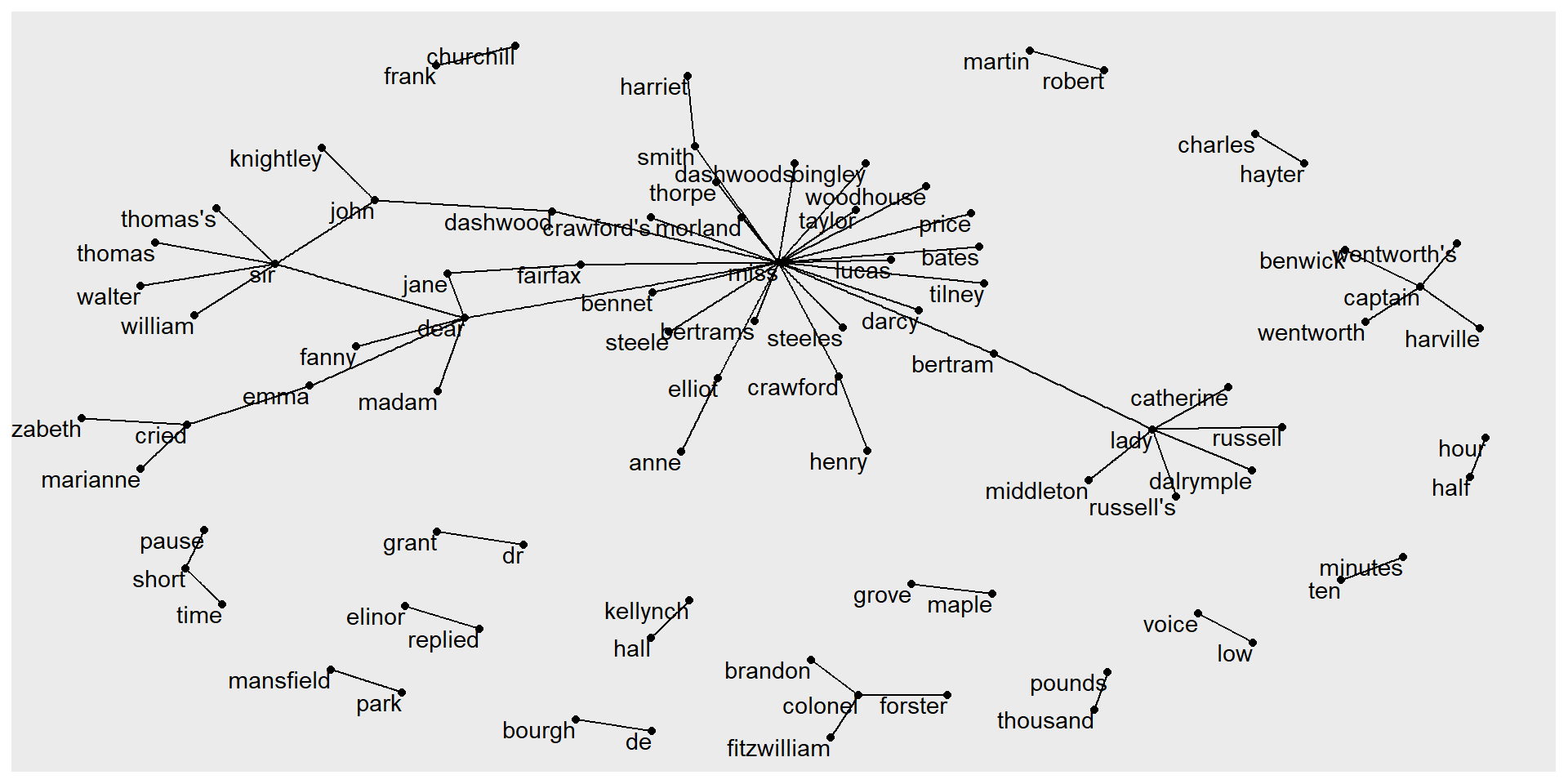
ggraph(bigram_graph, layout = "fr") +
  geom_edge_link() +  # draws edges
  geom_node_point() +  # draws nodes
  geom_node_text(aes(label = name), vjust = 1, hjust = 1) # adds labels

Make it fancy

a <- grid::arrow(type = "closed", length = unit(.15, "inches"))

ggraph(bigram_graph, layout = "fr") +
  geom_edge_link(aes(edge_alpha = n), show.legend = FALSE,
                 arrow = a, end_cap = circle(.07, "inches")) +
  geom_node_point(color = "lightblue", size = 5) +
  geom_node_text(aes(label = name), vjust = 1, hjust = 1) +
  theme_void()

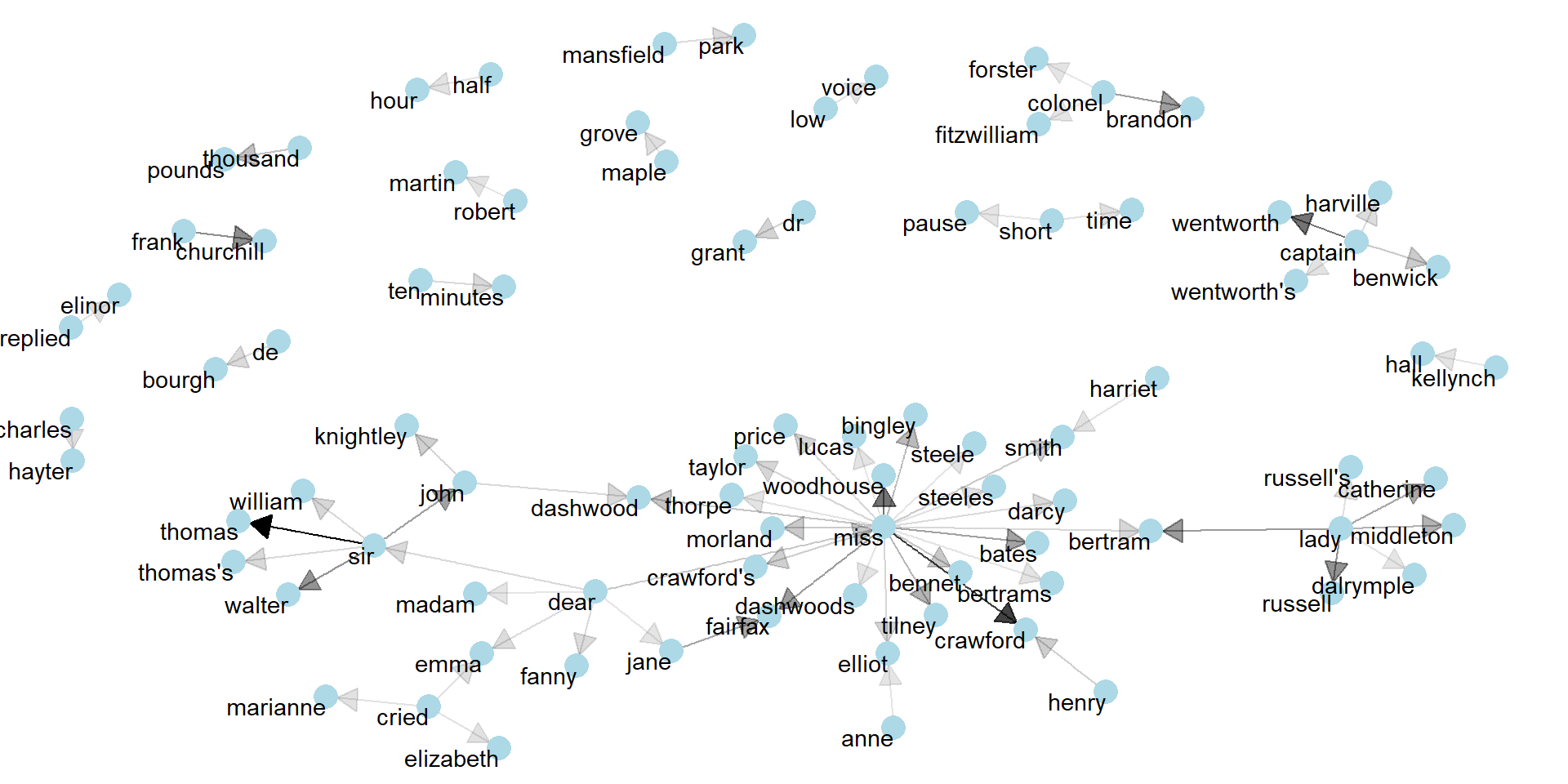
Arrows add direction, edge_alpha fades rarer bigrams, theme_void() strips the axes.

4.4 — Pairwise counts & correlations

Beyond adjacent words

• Bigrams only catch words that sit right next to each other
• Some words tend to show up in the same survey response, or the same stretch of an interview, without ever being adjacent
• the widyr package helps to find those co-occurrences (New package. Install when needed)

The textbook refers to the same passage - because they are analyzing books, not survey responses.

Splitting into sections

Pride & Prejudice has no natural sub-document smaller than a chapter, so we create an arbitrary 10-line window:

austen_section_words <- austen_books() |>
  filter(book == "Pride & Prejudice") |>
  mutate(section = row_number() %/% 10) |>
  filter(section > 0) |>
  unnest_tokens(word, text) |>
  filter(!word %in% stop_words$word)

head(austen_section_words)

# A tibble: 6 × 3
  book              section word        
  <fct>               <dbl> <chr>       
1 Pride & Prejudice       1 truth       
2 Pride & Prejudice       1 universally 
3 Pride & Prejudice       1 acknowledged
4 Pride & Prejudice       1 single      
5 Pride & Prejudice       1 possession  
6 Pride & Prejudice       1 fortune     

Choosing your section size

You may not have to manufacture this

• Survey free-response → a section is a single response. Each response is already a natural “document”.
• A whole transcript - you need to decide what the smaller unit is: a turn, a paragraph, or the same artificial-windowing trick shown here, depending on how your transcripts are structured.

Count co-occurring words in a ‘section’

Across every pair of distinct words, how many sections contain both words, regardless of where in sections they are or which came first.

word_pairs <- austen_section_words |>
  pairwise_count(word, section, sort = TRUE)

head(word_pairs)

# A tibble: 6 × 3
  item1     item2         n
  <chr>     <chr>     <dbl>
1 darcy     elizabeth   144
2 elizabeth darcy       144
3 miss      elizabeth   110
4 elizabeth miss        110
5 elizabeth jane        106
6 jane      elizabeth   106

Top pair: “darcy” and “elizabeth” — the two lead characters.

The problem with raw counts

word_pairs |>
  filter(item1 == "darcy") |> slice(1:5)

# A tibble: 5 × 3
  item1 item2         n
  <chr> <chr>     <dbl>
1 darcy elizabeth   144
2 darcy miss         92
3 darcy bingley      86
4 darcy jane         46
5 darcy bennet       45

“Darcy”/“Elizabeth” is the top pair mostly because both words are extremely common on their own — not because the pairing itself is special.

Warning: Math! 😱

	Has word Y	No word Y	Total
Has word X	\(n_{11}\)	\(n_{10}\)	\(n_{1\cdot}\)
No word X	\(n_{01}\)	\(n_{00}\)	\(n_{0\cdot}\)
Total	\(n_{\cdot 1}\)	\(n_{\cdot 0}\)	\(n\)

• \(n_{11}\) = sections where both words appear
• \(n_{00}\) = sections where neither appears
• \(n_{10}\)/\(n_{01}\) = sections where only one does.

\[ \phi = \frac{n_{11}n_{00} - n_{10}n_{01}}{\sqrt{n_{1\cdot}\, n_{0\cdot}\, n_{\cdot 0}\, n_{\cdot 1}}} \] The phi (\(\phi\)) coefficient asks: how much more likely are X and Y to appear together (or both be absent), compared to appearing separately? It’s equivalent to a Pearson correlation on binary data.

Calculating the \(\phi\) coefficient using R

word_cors <- austen_section_words |>
  group_by(word) |> filter(n() >= 20) |>
  pairwise_cor(word, section, sort = TRUE) # this calculates phi

head(word_cors)

# A tibble: 6 × 3
  item1    item2    correlation
  <chr>    <chr>          <dbl>
1 bourgh   de             0.951
2 de       bourgh         0.951
3 pounds   thousand       0.701
4 thousand pounds         0.701
5 william  sir            0.664
6 sir      william        0.664

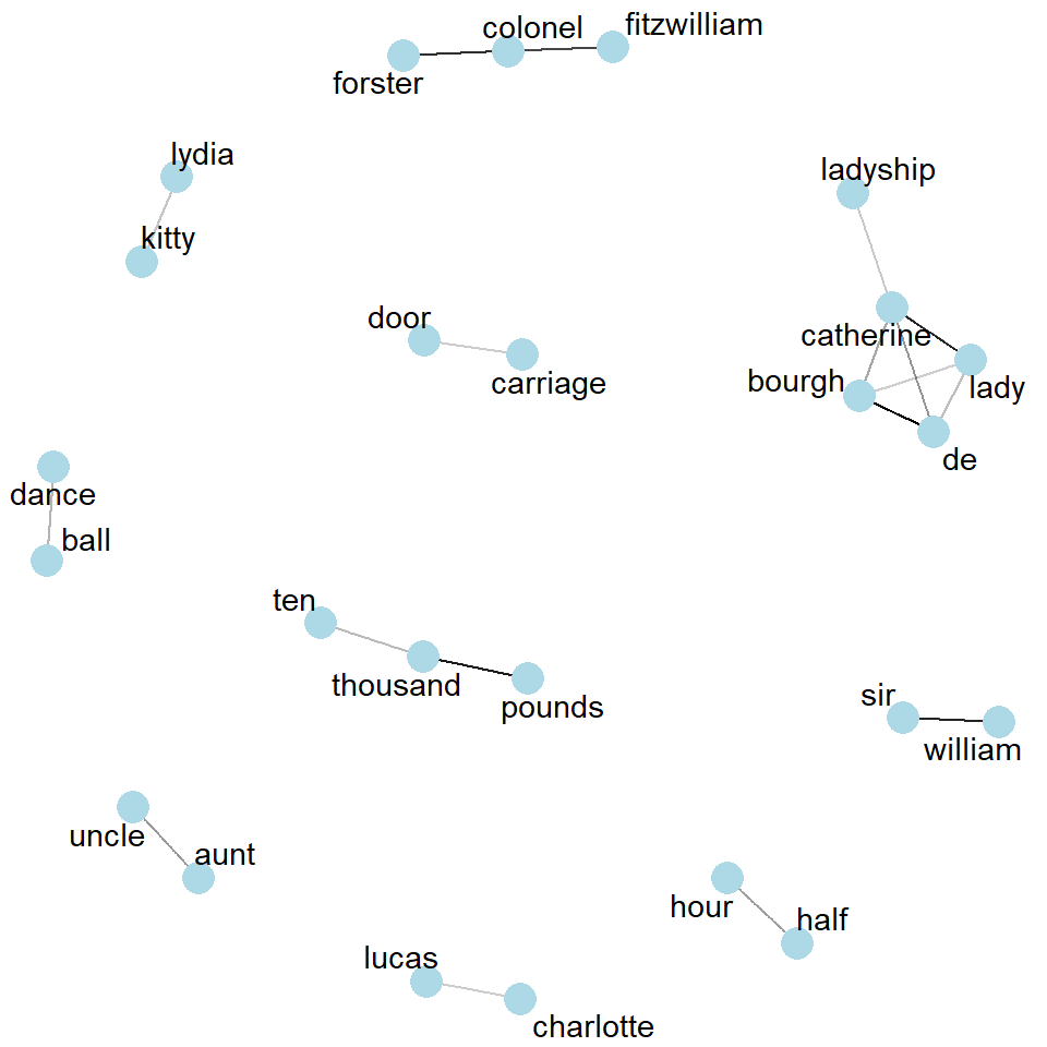
Now “bourgh”/“de” and “pounds”/“thousand” rise to the top — pairs that are rare individually but almost always appear together.

🎯 Your turn

Try it yourself

Filter word_cors for a word of your choice — item1 == "..." — and look at what it’s most correlated with. Does the result make sense?

Example:

word_cors |>
  filter(item1 == "pounds")

Visualizing correlations

word_cors |>
  filter(correlation > .25) |>
  graph_from_data_frame() |>
  ggraph(layout = "fr") +
  geom_edge_link(aes(edge_alpha = correlation), show.legend = FALSE) +
  geom_node_point(color = "lightblue", size = 5) +
  geom_node_text(aes(label = name), repel = TRUE) +
  theme_void()

We can use this \(\phi\) correlation value to filter a word network graph of pairs of words in Pride and Prejudice that show a co-occurrence correlation of at least .25 within the same 10-line section.

Wrap-up

Recap

• N-grams keep word order
• Bigrams give context: catching negation words like “not,” “no,” “never” fixes a real gap from last week
• We can visualize word pairs using a network — nodes, edges, and weights
• Word pairs often co-occur or correlate, even when they’re not adjacent