Sentiment Analysis
Code along 04
2026-09-21
Packages used for todays lesson
Learning objective
By the end of today, you’ll be able to:
- Attach a sentiment score to tidy text with
get_sentiments() - Compare how lexicons score the same passage
- Identify where dictionary-based methods break down — negation, context, domain-specific language
- Apply a sentiment score to an entire sentence
Tidying text recap
Last week you got text into tidy format and stripped out stop words:
tidy_books <- austen_books() |>  # get books
  group_by(book) |> # do separately for each book
  mutate(linenumber = row_number(), # add line numbers
         chapter = cumsum(str_detect(text, # and chapter numbers
                    regex("^chapter [\\divxlc]", ignore_case = TRUE)))) |>
  ungroup() |> # stop grouping by book
  unnest_tokens(word, text) |> # tokenize
  anti_join(stop_words) # remove stop words

head(tidy_books) # look at a few rows
# A tibble: 6 × 4
book linenumber chapter word
<fct> <int> <int> <chr>
1 Sense & Sensibility 1 0 sense
2 Sense & Sensibility 1 0 sensibility
3 Sense & Sensibility 3 0 jane
4 Sense & Sensibility 3 0 austen
5 Sense & Sensibility 5 0 1811
6 Sense & Sensibility 10 1 chapter Today - adding sentiment score to words
Once words carry a pos/neg tag, you can ask questions like
- “Do similar people share similar sentiments?”
- “Does the sentiment shift across an interview?”
2.1 — The sentiment lexicons
Three general-purpose lexicons
- These lexicons are based on unigrams, i.e., single words.
- These lexicons contain many English words and the words are assigned scores for positive/negative sentiment,
- and also possibly emotions like joy, anger, sadness, and so forth.
Load sentiment lexicons - First time each session
We run get_sentiments("lexicon name") to load in the lexicon through the textdata package. This may prompt to confirm a download the first time they’re called in a session.
Lets look at each one first.
bing
Liu et al. — binary: positive or negative
nrc
Mohammad & Turney — 10 categories: positive, negative, anger, anticipation, disgust, fear, joy, sadness, surprise, trust
AFINN
Nielsen — numeric score. -5 (very negative) to +5 (very positive)
⚠️ Two caveats
- No negation handling — these are unigram methods. Once “not true” is split into two tokens, “true” just looks true. The qualifier in front of it is invisible to a word-level join
- Chunk size matters — score a whole multi-paragraph document and positive/negative words often cancel out to ~zero. Sentence- or paragraph-sized chunks score better
2.2 — Sentiment analysis with inner_join()
The core pattern
This time we keep the matches instead of dropping them. So only words with sentiments are retained.
# A tibble: 6 × 5
  book                linenumber chapter word        sentiment
  <fct>                    <int>   <int> <chr>       <chr>
1 Sense & Sensibility         16       1 respectable positive
2 Sense & Sensibility         18       1 advanced    positive
3 Sense & Sensibility         20       1 death       negative
4 Sense & Sensibility         21       1 loss        negative
5 Sense & Sensibility         25       1 comfortably positive
6 Sense & Sensibility         28       1 goodness    positive
Joy in Emma
# A tibble: 297 × 2
   word          n
   <chr>     <int>
 1 friend      166
 2 hope        143
 3 happy       125
 4 love        117
 5 deal         92
 6 found        92
 7 happiness    76
 8 pretty       68
 9 true         66
10 comfort      65
# ℹ 287 more rows
Look closely: “found” and “present” are in there too — not exactly overflowing with joy.
🎯 Your turn
Try it yourself
Find the "trust" words in "Pride & Prejudice" using the nrc lexicon.
Answer
# A tibble: 405 × 2
   word         n
   <chr>    <int>
 1 hope       121
 2 father     116
 3 mother     112
 4 friend     104
 5 happy       83
 6 aunt        78
 7 sir         78
 8 brother     66
 9 found       66
10 marriage    66
# ℹ 395 more rows
2.3 — Comparing three lexicons
Same passage, three scorers
- This example uses Emma chapter 1
- Score the exact same words with AFINN, bing, and NRC
- Compare which words each lexicon treats as meaningful
AFINN: frequency and score
Create a new variable contribution as the frequency of word occurrence (n) times the numeric sentiment value of the word.
# A tibble: 6 × 4
  word      value     n contribution
  <chr>     <dbl> <int>        <dbl>
1 miss         -2    26          -52
2 poor         -2    11          -22
3 dear          2     9           18
4 success       2     6           12
5 pretty        1     5            5
6 affection     3     4           12
Plot AFINN
Is there a strong sentiment (repeated positive or negative words) in this chapter?
Code
afinn_words |>
  mutate(label = if_else(abs(contribution) >= 6, word, "")) |>
  ggplot(aes(n, value, color = value > 0, size = abs(contribution))) +
  geom_point(alpha = 0.75, show.legend = FALSE) +
  geom_text(aes(label = label), check_overlap = TRUE,
            show.legend = FALSE, vjust = -0.7) +
  scale_y_continuous(breaks = -5:5) +
  labs(x = "Count in chapter", y = "AFINN score")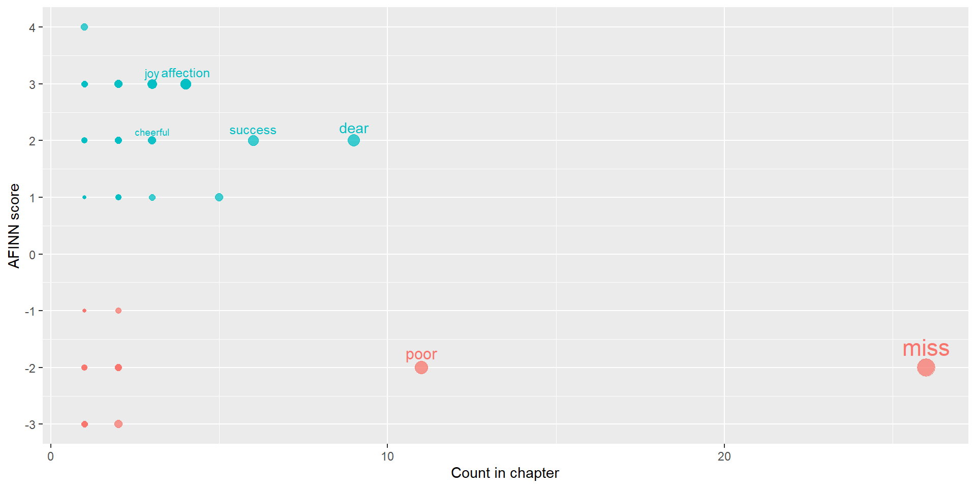
Bing: positive and negative words
Count the number of times the words appear, but now the sentiment is added.
# A tibble: 6 × 3
  word      sentiment     n
  <chr>     <chr>     <int>
1 miss      negative     26
2 poor      negative     11
3 success   positive      6
4 pretty    positive      5
5 affection positive      4
6 lucky     positive      4
Plot Bing
Allowing us to compare the most frequent positive and negative words.
Code
bing_words |>
  group_by(sentiment) |>
  slice_max(n, n = 5) |>
  ungroup() |>
  mutate(word = reorder_within(word, n, sentiment)) |>
  ggplot(aes(n, word, fill = sentiment)) +
  geom_col(show.legend = FALSE) +
  facet_wrap(~sentiment, scales = "free_y") +
  scale_y_reordered() +
  labs(x = "Count in chapter", y = NULL)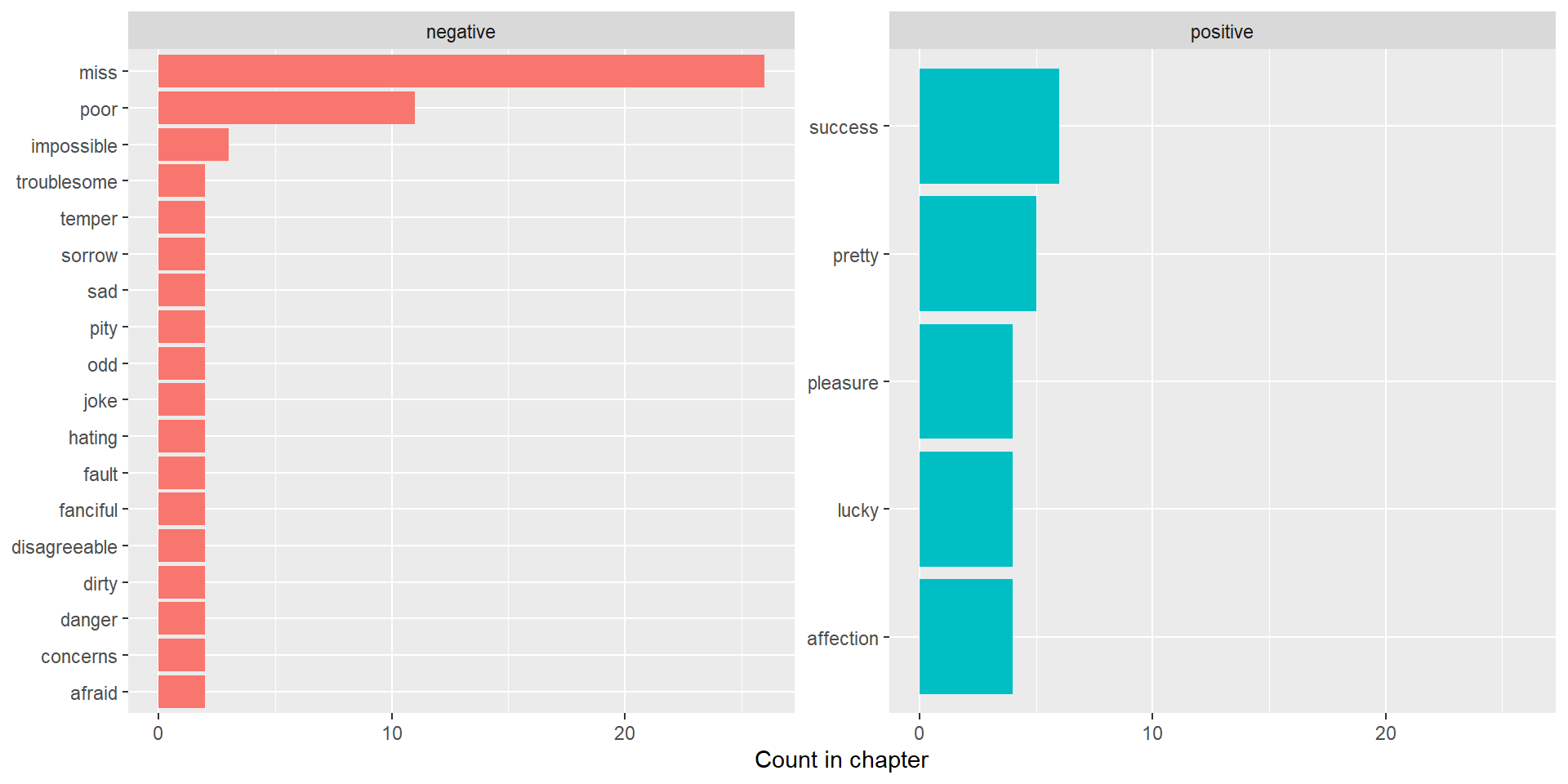
NRC: ten categories
Plot NRC
Code
nrc_words |>
  group_by(sentiment) |>
  slice_max(n, n = 5) |>
  ungroup() |>
  mutate(word = reorder_within(word, n, sentiment)) |>
  ggplot(aes(n, word, fill = sentiment)) +
  geom_col(show.legend = FALSE) +
  facet_wrap(~sentiment, scales = "free_y", nrow=2) +
  scale_y_reordered() +
  labs(x = "Count in chapter", y = NULL)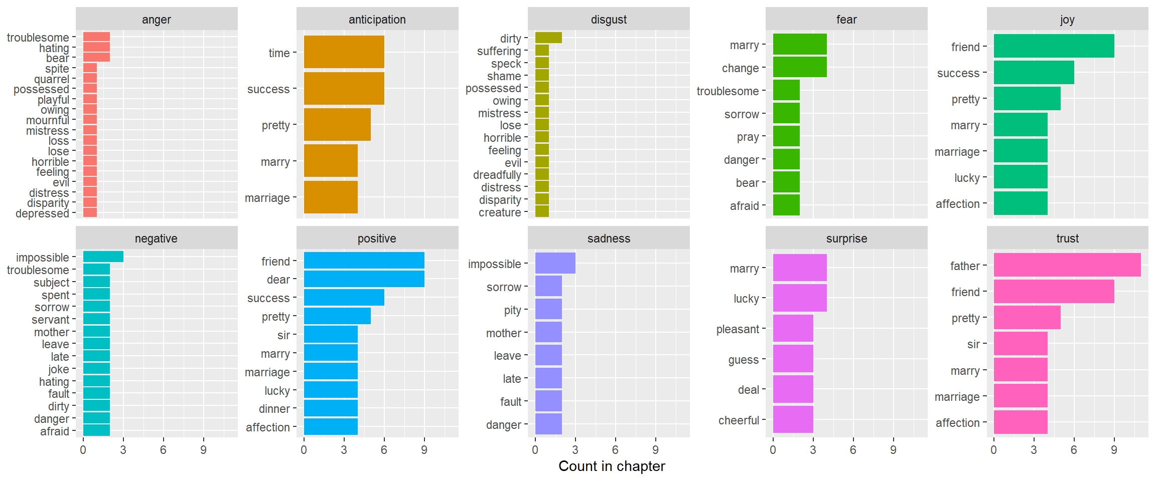
Reading across lexicons
Same text, different measuring tools.
- AFINN shows both how often a word appears and how strongly it is scored
- Bing asks a simpler question: which words count as positive or negative?
- NRC spreads the same chapter across emotion categories, so a word can appear in more than one facet
Lexicon balance
# A tibble: 4 × 3
  sentiment     n lexicon
  <chr>     <int> <chr>
1 negative   4781 bing
2 positive   2005 bing
3 negative   3316 nrc
4 positive   2308 nrc
That means the “same” passage can look different before we even get to questions of context.
2.4 — Check the words, not just the score
🚩 Wait — “miss”?
- In Austen’s world, Miss is often a title for an unmarried woman
- Stripped of context, this looks negative to bing. The lexicon has no way to know it is a title in this text.
- A general-purpose dictionary can’t account for context-specific meaning
🎯 Your turn — fix it
Try it yourself
Add "miss" to a custom stop-word list (same pattern as last week), rebuild bing_words, and see the negative counts change.
2.6 — Sentence-level sentiment
Score whole sentences
- Instead of scoring isolated words, score whole sentences
- A sentence keeps nearby context available to the sentiment algorithm
- The important question: does the algorithm actually use that context?
Valence shifters
- Negators:
not happy - Amplifiers:
very happy - De-amplifiers:
barely happy - Adversative conjunctions:
happy, but worried
Sentence scores with sentimentr
The single sentiment() function tokenizes on sentences AND calculates a sentence level score.
Key: <element_id, sentence_id>
   element_id sentence_id word_count   sentiment
        <int>       <int>      <int>       <num>
1:          1           1          6  0.30618622
2:          2           1          7 -0.28347335
3:          2           2          2 -0.35355339
4:          3           1          7  0.51025204
5:          3           2          2  0.00000000
6:          4           1          7  0.05669467
7:          4           2          2  0.00000000
8:          5           1         11 -0.18844459
9:          5           2          2 -0.53033009
Apply it to Austen
Add a couple data wrangling steps so we can see the sentences along with the scores.
1pp_sentences <- get_sentences(prideprejudice) |> unlist()

2p_and_p_sentences <- tibble(sentence_id = seq_along(pp_sentences),
                            sentence = pp_sentences)

3scores <- sentiment(p_and_p_sentences$sentence) |>
  mutate(sentence_id = element_id) |>
  select(sentence_id, score = sentiment)

4pp_sentence_scores <- p_and_p_sentences |>
left_join(scores, by = "sentence_id")- 1
- tokenize the book into sentences
- 2
- convert to a data frame for later merging
- 3
- apply the sentiment score, keep only sentence id and sentiment score
- 4
- merge sentences back onto scores
Most negative sentences
[1] "Elizabeth lifted up her eyes in amazement, but was too much oppressed"
[2] "only one who shed tears; but she did weep from vexation and envy."
[3] "ached acutely."
[4] "most disagreeable."
[5] "sure it will be too much for Kitty." Sentence and score shown in two steps due to word wrapping.
Most positive sentences
[1] "chosen so much more advantageously in many respects."
[2] "more pleasant aspect; but she soon saw that her friend had an excellent"
[3] "But gracious"
[4] "\"Yes, very handsome.\""
[5] "acceptance of the invitation was most ready and grateful." What this gives us
- Sentence-level scores are better for local context
- They still do not understand sarcasm, irony, speaker intent, or domain-specific meaning
- Use them to find places worth reading closely, not as a replacement for interpretation
- Sentence tokenizing is not perfect, especially with dialogue, abbreviations, and unusual punctuation.
Recap
- Sentiment lexicons attach a pos/neg (or emotion) label per word, joined the same way you joined out stop words
- Different lexicons can highlight different words in the same passage
- The best check is often a word-level plot: which words are driving the score?