Helper code
How do I…?
This helper page provides additional code examples to accomplish tasks that we won’t get a chance to discuss directly during class time. All code examples uses the data from the Day 1 survey
But first, a message from our sponsors….
1 Additional learning materials
- General R
- Start with Math 130: https://math130.netlify.app
- Move to R for Data Science: https://r4ds.hadley.nz/
- Factors (intentionally managed categorical variables)
-
forcatspackage vignette: https://forcats.tidyverse.org/articles/forcats.html
-
- String manipulation
-
stringrpackage vignette: https://stringr.tidyverse.org/articles/stringr.html
-
- Plotting
- Inspiration from the R graph gallery: https://r-graph-gallery.com/
- Ggplot2 cookbook https://r-graphics.org/
- Do more with Quarto: https://quarto.org/docs/gallery/
2 Variable Names
Sometimes the names of the questions are too long. This is most often the case if you are using data collected from a Google Form.
names(survey)[1] "Where are you from?"
[2] "How much experience do you have with programming?"
[3] "How much experience do you have with qualitative research, broadly (e.g. project conceptualization, identifying a sampling strategy, interview instrument design, survey design, data management, etc.)?"
[4] "How much experience do you have with qualitative data analysis, specifically (e.g. grounded theory, open coding, focused coding, concept mapping, memoing, Dedoose software, theme generation, writing findings, etc.)?"
[5] "What types of data interest you?"
[6] "How do you learn best?"
[7] "What do you hope to get out of this course?" 2.1 Rename all variables by position
You can overwrite the names() of the data by providing a vector of new names - but order that you specify the new variable names is critical here. It must match the order found in the data set.
2.2 Rename only a few variables
We can also use the rename(new name = old name) function.
3 Data management
These are the basic functions for checking, sorting, and summarizing a data set. The examples use counts, the number of students in each location.
counts <- count(survey, location)
counts
# A tibble: 5 × 2
location n
<chr> <int>
1 Broader North State (Sac & up) 4
2 Butte County 6
3 Outside of the United States 2
4 Rest of California 5
5 United States - Outside California 3| I want to… | Function and example | Watch for |
|---|---|---|
| Know how many rows or columns |
nrow(survey), ncol(survey)
|
nrow(counts) is the number of groups |
| Count how many in each group | count(survey, location) |
The new column is called n. sort = TRUE puts the biggest first. |
| Make a quick table, or cross two variables |
table(survey$location), table(survey$location, survey$programming_experience)
|
It isn’t a data frame, so you can’t pipe it into filter() and friends. useNA = "always" shows missing values. |
| Sort rows |
arrange(counts, n), arrange(counts, desc(n))
|
desc() puts the biggest first |
| Look at the first few rows | head(survey, 3) |
The default is 6. After arrange(), it shows the top or bottom. |
| Keep rows that meet a condition | filter(survey, location == "Butte County") |
== equal, != not equal, > greater, & and. For “or” across several values, see the next row. |
| Match any of several values | filter(survey, location %in% c("Butte County", "Rest of California")) |
Shorter than writing one == test per value |
| Keep the row with the biggest value | slice_max(counts, n, n = 1) |
After group_by() it keeps the biggest in each group, so add ungroup(). Ties are all kept. |
| Find missing values |
filter(survey, is.na(location)), sum(is.na(survey$location))
|
sum() counts the TRUEs |
| Get the smallest, largest, and average | summarize(counts, smallest = min(n), largest = max(n), avg = mean(n)) |
One row comes out |
| Total within groups | summarize(group_by(counts, location), people = sum(n)) |
group_by() first gives one row per group |
| Pull one value out of a data frame | counts$n[1] |
$ gives a column; [1] takes its first value |
| Add columns from another table | left_join(survey, counts, by = "location") |
Keeps every row of the first table. If the key columns have different names, use by = c(document = "exhibit"). |
| List the distinct values as one string | paste(unique(survey$location), collapse = "; ") |
unique() drops repeats; collapse glues the values together |
4 Identifying records with key words.
Consider the data_interests “select all that apply” question. Each response is one string with the choices separated by ;, so we can’t just count how many people picked “Health”. We need a way to search through their responses to find specific topics.
# A tibble: 6 × 1
  data_interests
  <chr>
1 Health; No preference
2 Sports; Health
3 Education; Politics
4 Crime; Economics
5 Health; Education
6 Environment/Climate; Politics
The general tactic is to create a new variable that is an indicator for whether or not the keyword is in that variable text. This can also be called a binary indicator because it only has two options TRUE if the keyword was found, and FALSE if it was not found.
4.1 One keyword
str_detect(x, pattern) looks inside every value of the variable x and returns TRUE if the pattern is found, FALSE if not.
survey <- survey |>
  mutate(int_health = str_detect(data_interests, "Health"))

survey |>
  select(data_interests, int_health) |>
  head()
# A tibble: 6 × 2
data_interests int_health
<chr> <lgl>
1 Health; No preference TRUE
2 Sports; Health TRUE
3 Education; Politics FALSE
4 Crime; Economics FALSE
5 Health; Education TRUE
6 Environment/Climate; Politics FALSE 4.2 Several keywords
Use | inside the pattern to mean “or”. This flags students who picked Crime or Politics.
survey <- survey |>
  mutate(crime_or_politics = str_detect(data_interests, "Crime|Politics"))

survey |>
  select(data_interests, crime_or_politics) |>
  head()
# A tibble: 6 × 2
data_interests crime_or_politics
<chr> <lgl>
1 Health; No preference FALSE
2 Sports; Health FALSE
3 Education; Politics TRUE
4 Crime; Economics TRUE
5 Health; Education FALSE
6 Environment/Climate; Politics TRUE For “and”, use two str_detect() calls joined with &. This flags students who picked Politics and Economics.
survey <- survey |>
  mutate(politics_and_econ = str_detect(data_interests, "Politics") &
                             str_detect(data_interests, "Economics")
         )

survey |>
  select(data_interests, politics_and_econ) |>
  slice(16:20)
# A tibble: 5 × 2
data_interests politics_and_econ
<chr> <lgl>
1 Politics; Economics; Sports TRUE
2 Health; No preference FALSE
3 Economics; Crime FALSE
4 Sports FALSE
5 Politics; Economics; Education TRUE Watch out
str_detect() is case sensitive: "health" will not find "Health". Wrap the pattern in regex() to ignore case.
survey |> summarise(
  exact       = sum(str_detect(data_interests, "health")),
  ignore_case = sum(str_detect(data_interests,  regex("health", ignore_case = TRUE)))
  )
4.3 Multiple indicators at once
You can create multiple new indicator variables in a single mutate statement.
survey <- survey |>
  mutate(
    int_education = str_detect(data_interests, "Education"),
    int_politics  = str_detect(data_interests, "Politics"),
    int_economics = str_detect(data_interests, "Economics"),
    int_sports    = str_detect(data_interests, "Sports")
  )
5 Wrangling Categorical Variables
5.1 Shortening response options
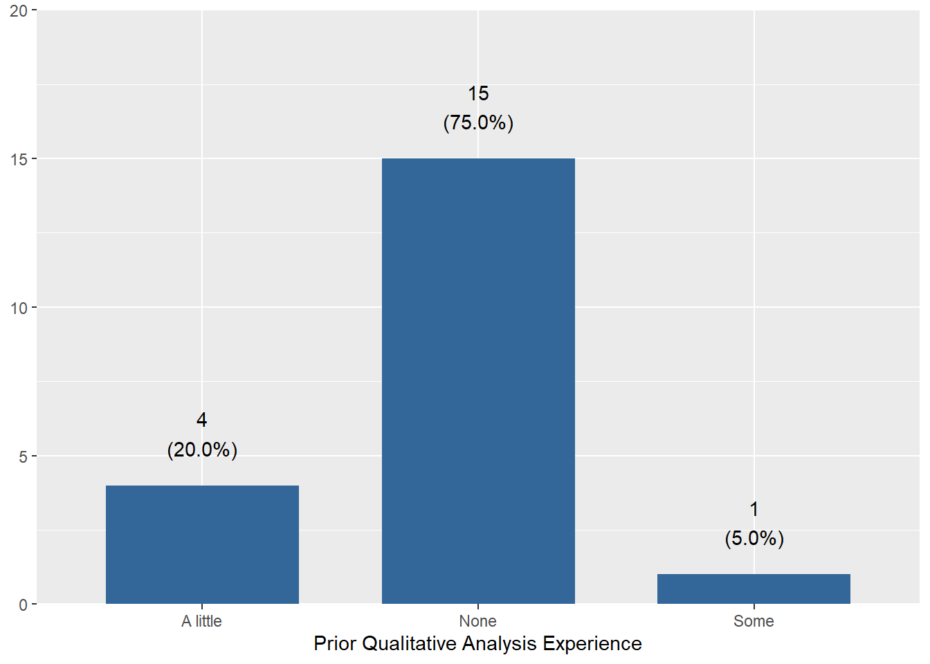
Problem. qual_dta asks about prior experience with qualitative data analysis (coding, memoing, theme generation, etc.). The answers are long text, which can result in word wrapping problems.
table(survey$qual_dta)
      A little - for example, I have taken a research methods class where we were taught qualitative data analysis
                                                                                                                 4
                                                                                                              None
                                                                                                                15
Some - I've worked on at least one project where I have had to practice some elements of qualitative data analysis
                                                                                                                 1
Solution Make a new variable using mutate that shortens the response labels manually. The case_when() function says “if you see the words on the left, then write the thing on the right”. The TRUE at the end allows other levels to remain unchanged. In this case, the “None” level doesn’t get changed.
survey <- survey %>%
  mutate(qda = case_when(
    qual_dta == "A little - for example, I have taken a research methods class where we were taught qualitative data analysis" ~ "A little",
    qual_dta == "Some - I've worked on at least one project where I have had to practice some elements of qualitative data analysis" ~ "Some",
    TRUE ~ qual_dta)
  )

survey %>% count(qual_dta, qda)
# A tibble: 3 × 3
qual_dta qda n
<chr> <chr> <int>
1 A little - for example, I have taken a research methods class whe… A li… 4
2 None None 15
3 Some - I've worked on at least one project where I have had to pr… Some 1Watch out
When changing response levels like this, always make a new variable to hold the changed values. This way you can visually confirm that the changes you made actually work. And when you mess up, because everyone does, you didn’t mess up the original variable.
Always trust, but verify your coding worked as intended.
table(survey$qda, useNA="always")
A little     None     Some     <NA>
       4       15        1        0
5.2 Collapse a factor into fewer categories
Problem. location has five categories and two of them have only 2 or 3 students. We’d like fewer, larger groups.
survey |>
  count(location)
# A tibble: 5 × 2
location n
<chr> <int>
1 Broader North State (Sac & up) 4
2 Butte County 6
3 Outside of the United States 2
4 Rest of California 5
5 United States - Outside California 35.2.1 Collapse the levels
We’ll use the fct_collapse() from the forcats package (loaded with tidyverse). This function takes "new name" = c("old level", "old level") pairs.
survey <- survey |>
  mutate(location_grp = fct_collapse(location,
    "North State"        = c("Butte County", "Broader North State (Sac & up)"),
    "Outside California" = c("United States - Outside California",
                             "Outside of the United States")
  ))
Trust, but verify
table(survey$location, survey$location_grp, useNA = "always")
                                     North State Outside California
  Broader North State (Sac & up)               4                  0
  Butte County                                 6                  0
  Outside of the United States                 0                  2
  Rest of California                           0                  0
  United States - Outside California           0                  3
  <NA>                                         0                  0

                                     Rest of California <NA>
  Broader North State (Sac & up)                      0    0
  Butte County                                        0    0
  Outside of the United States                        0    0
  Rest of California                                  5    0
  United States - Outside California                  0    0
  <NA>                                                0    0
The 6 Butte and 4 broader north state are now just north state, the 2 Outside US and 3 outside CA are just outside CA, and the rest of CA remained unchanged.
5.2.2 Put the new levels in order
The new levels come out in alphabetical order, which may not be desirable. Use fct_relevel() to list the levels in the order you want.
survey <- survey |>
  mutate(location_grp = fct_relevel(location_grp,
                                    "North State", "Rest of California", "Outside California"))

table(survey$location_grp)
       North State Rest of California Outside California
                10                  5                  5
6 Plotting
6.1 Resize graphics
We’ll use a simple bar chart of qualitative data analysis experience, made with plot_frq() from the sjPlot package. By default Quarto makes figures 7 inches wide by 5 inches tall.
6.1.1 fig-width and fig-height
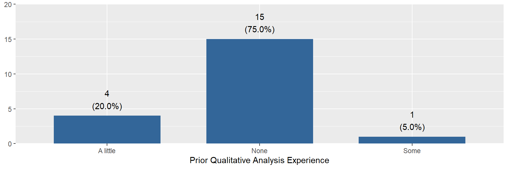
Set the size in inches with chunk options (lines that start with #| at the top of the chunk). Below, echo: fenced shows the whole chunk, including the options, so you can see what was typed.
```{r}
#| fig-width: 9
#| fig-height: 3
#| fig-alt: "The same bar chart drawn wide and short."
plot_frq(survey, qda) + labs(x = "Prior Qualitative Analysis Experience")
```
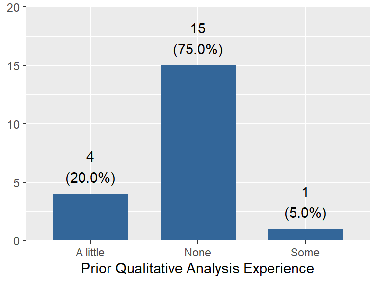
```{r}
#| fig-width: 4
#| fig-height: 3
#| fig-alt: "The same bar chart drawn small."
plot_frq(survey, qda) + labs(x = "Prior Qualitative Analysis Experience")
```
Watch out
Text size is fixed in points, so it doesn’t grow with the figure. A bigger figure makes the text look smaller relative to the plot, and a smaller figure makes it look bigger. Make it too small and labels start to collide or get cut off.
If you render to PDF, the text area is only about 6 inches wide. A figure wider than that is shrunk to fit, and the text shrinks with it.
6.1.2 out-width and fig-align
out-width leaves the plot as drawn and scales the finished picture on the page. fig-align positions it.
```{r}
#| out-width: "60%"
#| fig-align: center
#| fig-alt: "The same bar chart displayed at 60 percent of the page width."
plot_frq(survey, qda) + labs(x = "Prior Qualitative Analysis Experience")
```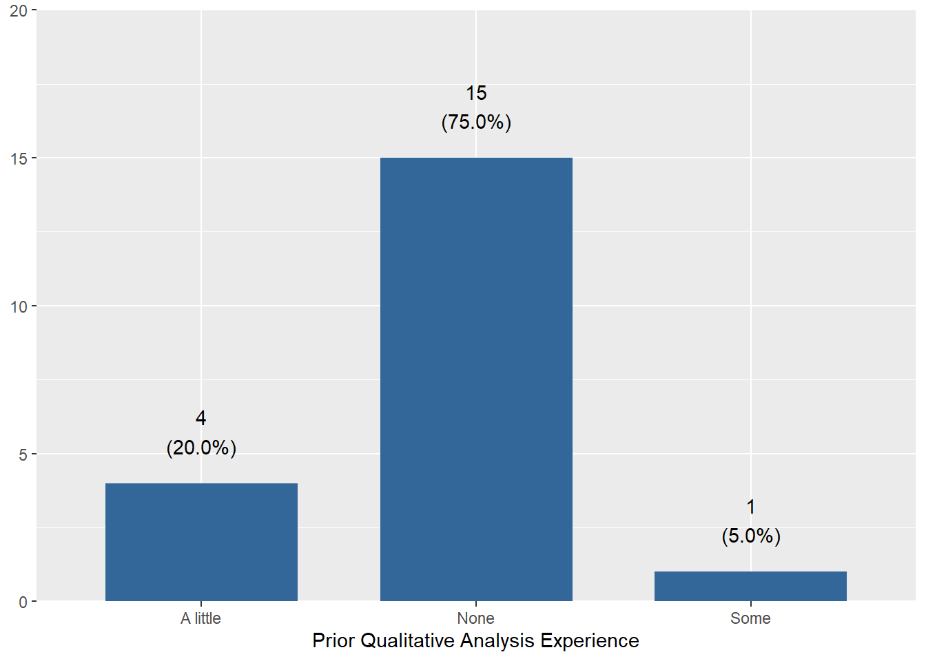
Use fig-width/fig-height to change the shape of the plot. Use out-width to change how much room it takes on the page.
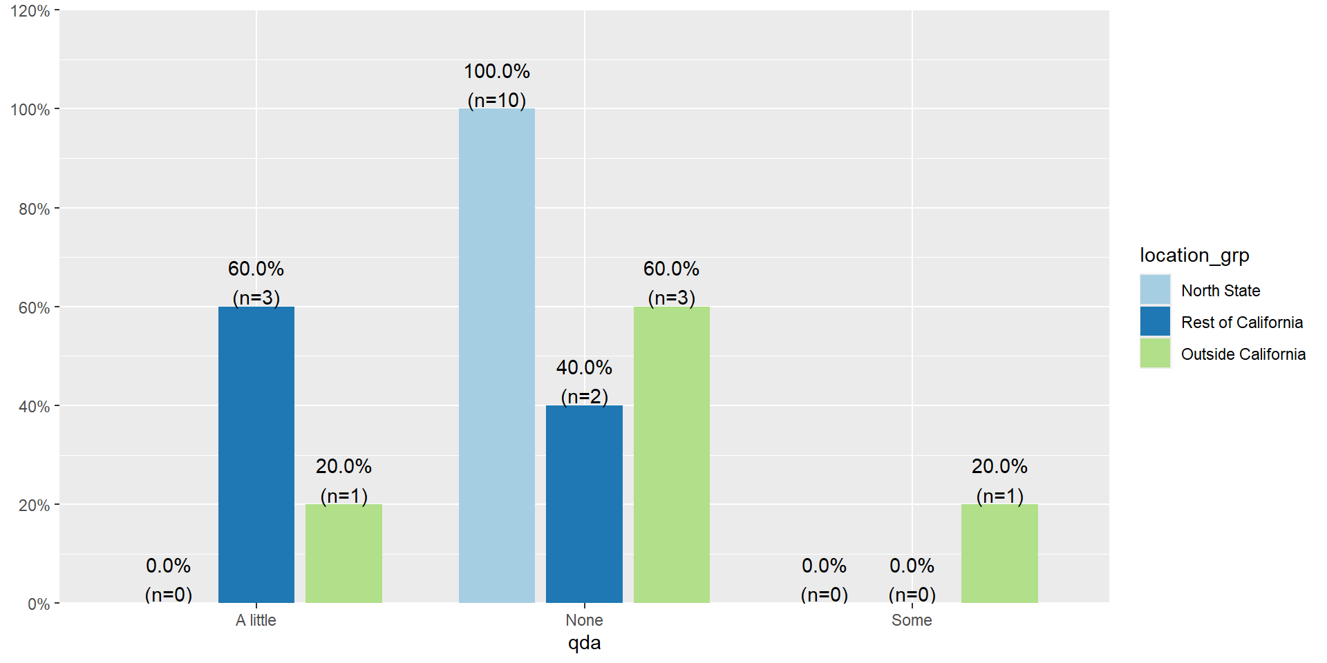
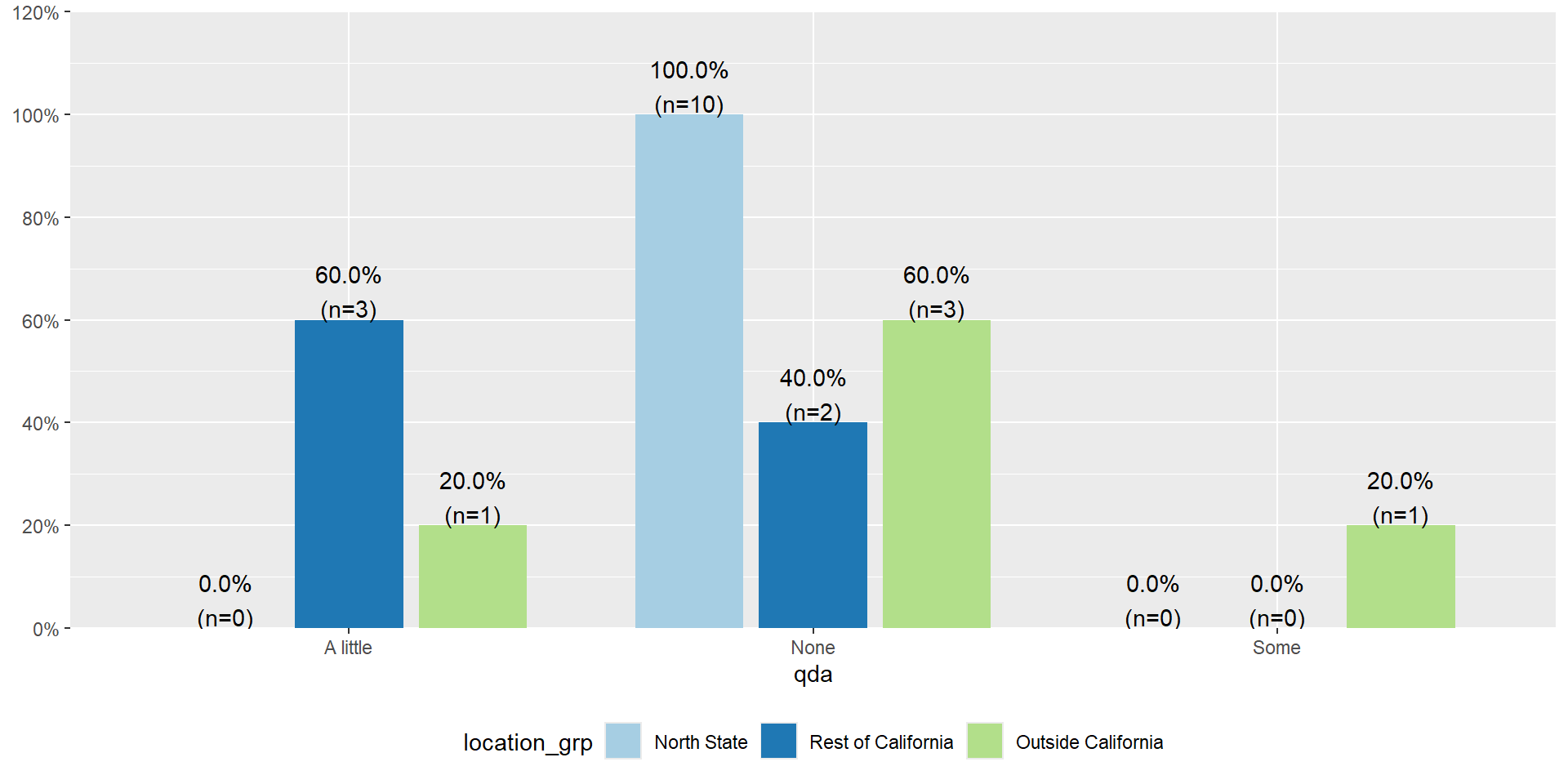
6.2 Modifying the legend
The legend goes on the right by default. legend.position accepts "top", "bottom", "left", "right" and "none". Use legend.position = "none" when the colors are already explained somewhere else, such as direct labels on the plot or the axis.
6.3 Adding Figure Captions
Figures produced by executable code blocks are automatically included in your document. To set the ID and caption and link, use the chunk options label and fig-cap respectively.
You can also create subcaptions for computational output by combining the fig-cap and fig-subcap options. When applying captions to computational output you can optionally include a label with a fig- prefix—if you do this then the figure will be numbered and cross-referenceable.
```{r}
#| fig-height: 5
#| fig-width: 10
#| layout-ncol: 2
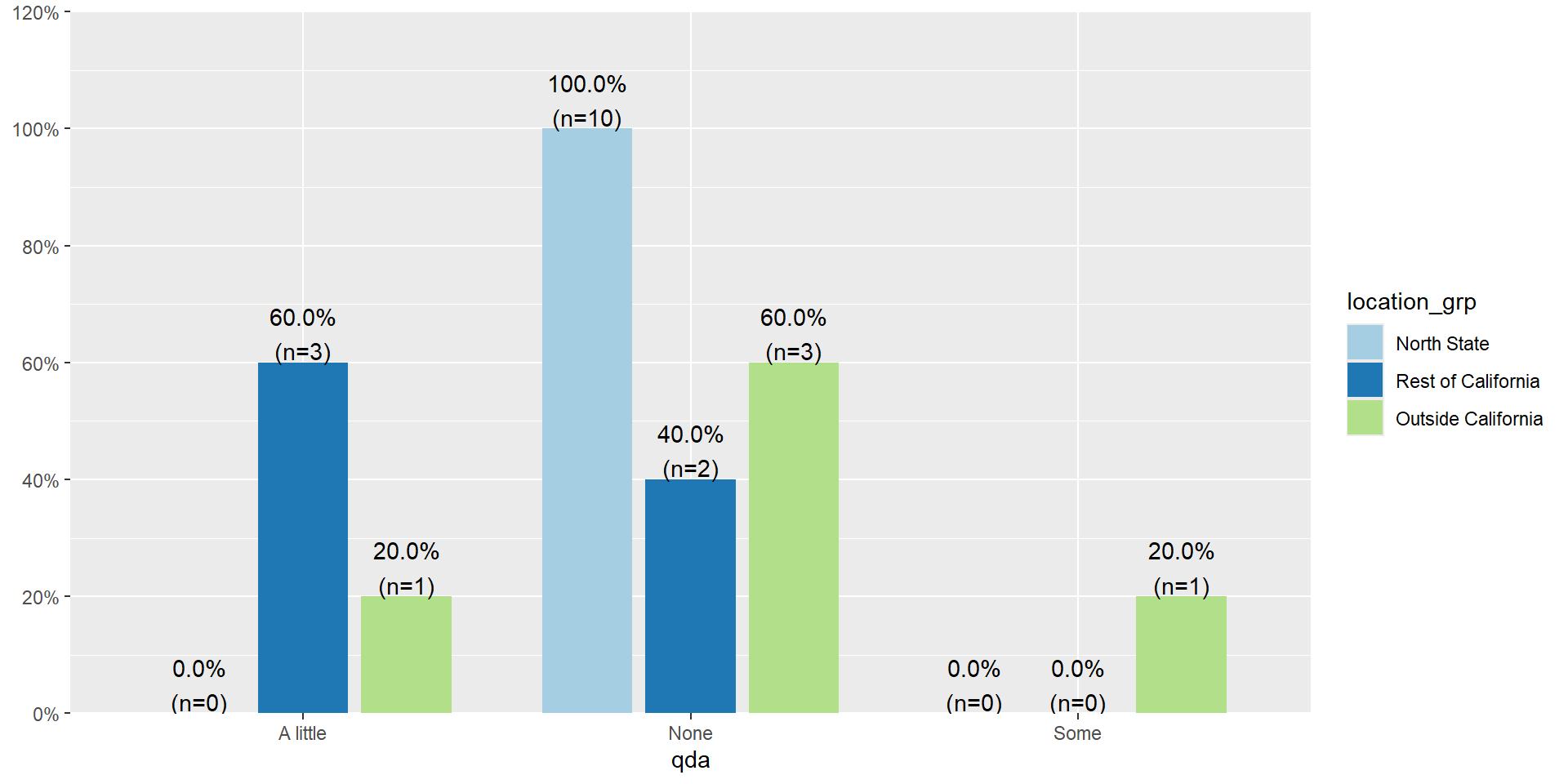
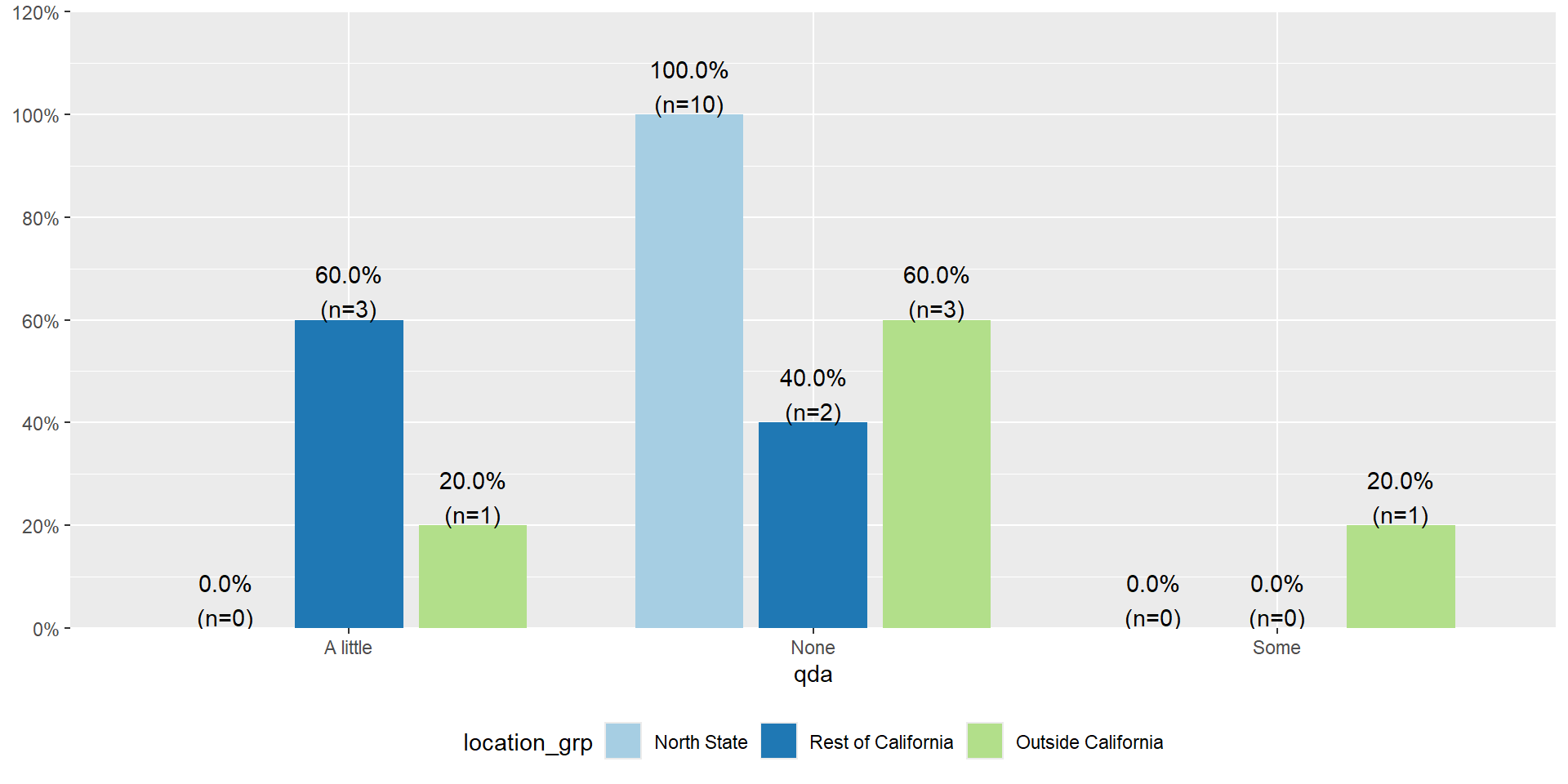
#| fig-cap: "Legend modifications"
#| fig-subcap:
#| - "Default legend location"
#| - "Legend at bottom"
plot_xtab(survey$qda , grp = survey$location_grp, show.total = FALSE)
plot_xtab(survey$qda , grp = survey$location_grp, show.total = FALSE) +
  theme(legend.position = "bottom")
```
Legend modifications